Optoelectronic reservoir computing

Abstract

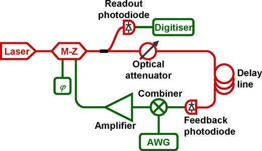
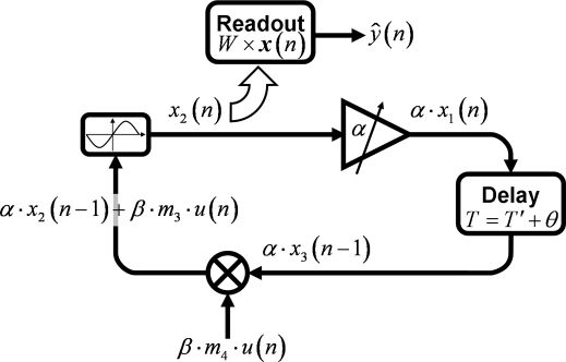
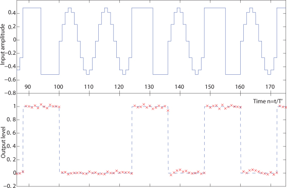
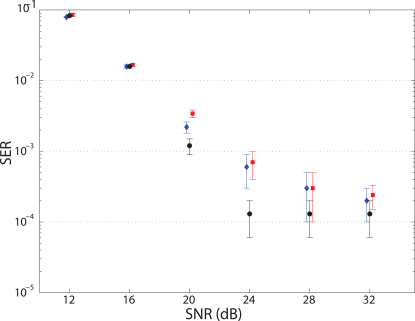
Reservoir computing is a recently introduced, highly efficient bio-inspired approach for processing time dependent data. The basic scheme of reservoir computing consists of a non linear recurrent dynamical system coupled to a single input layer and a single output layer. Within these constraints many implementations are possible. Here we report an optoelectronic implementation of reservoir computing based on a recently proposed architecture consisting of a single non linear node and a delay line. Our implementation is sufficiently fast for real time information processing. We illustrate its performance on tasks of practical importance such as nonlinear channel equalization and speech recognition, and obtain results comparable to state of the art digital implementations.

Figure 1. Schematic of the experimental set-up.

The red and green parts represent respectively the optical and electronic components. The optical part of the setup is fiber based, and operates around 1550 nm (standard telecommunication wavelength). “M-Z”: Lithium Niobate Mach-Zehnder modulator. “ϕ”: DC voltage determining the operating point of the M-Z modulator. “Combiner” : electronic coupler adding the feedback and input signals. “AWG”: arbitrary waveform generator. A computer generates the input signal for a task and feeds it into the system using the arbitrary waveform generator. The response of the system is recorded by a digitiser and retrieved by the computer which optimizes the read-out function in a post processing stage. The feedback gain α is adjusted by changing the average intensity inside the loop with the optical attenuator. The input gain β is adjusted by changing the output voltage of the function generator by a multiplicative factor. The bias ϕ is adjusted by using a DC voltage to change the operating point of the M-Z modulator. The operation of the system is fully automated and controlled by a computer using MATLAB scripts.

Figure 2. Schematic diagram of the information flow in the experiment depicted in Fig. 1.

On the plot we have represented four reservoir nodes at different stages of processing, labeled according to equation 5 with k = 1. Starting from the bottom, and going clockwise, a input value u(n) gets multiplied by an input gain β and a mask value m_i, then mixed with the previous node state αx_i−k(n − 1). The result goes through the sine function to give the new state of the reservoir x_i(n), which then gets amplified by a factor α and, after the delay, will get mixed with a new input u(n + 1). All the network states x_i(n) are also collected by the readout unit, multiplied by their respective weights W_i and added together to give the desired output ŷ(n).

Figure 3. Signal classification task.

The aim is to differentiate between square and sine waves. The top panel shows the input u(t), a stepwise constant function resulting from the discretization of successive step and sine functions. The bottom panel shows in red crosses the output of the reservoir ŷ (n). The target function (dashed line in the lower panel) is equal to 1 when the input signal is a step function and to 0 when the input signal is a sine function. The Normalized Mean Square Error, evaluated over 1000 inputs, is .

Figure 4. Results for nonlinear channel equalization.

The horizontal axis is the Signal to Noise Ratio (SNR) of the channel. The vertical axis is the Symbol Error Rate (SER), that is the fraction of input symbols that are misclassified. Results are plotted for the experimental setup (black circles), the discrete simulations based on eq. (5) (blue rhomboids), and the continuous simulations that take into account noise and bandpass filters in the experiment (red squares). All three sets of results agree within the statistical error bars. Error bars on the experimental points relative to 24, 28 and 32 dB might be only roughly estimated (see Supplementary Material). The results are practically identical to those obtained using a digital reservoir in.

References

1. Caulfield H. J. & Dolev S. Why future supercomputing requires optics. Nature Photon. 4 261–263 (2010).
1. Jaeger H. The “echo state” approach to analysing and training recurrent neural networks. Technical Report GMD Report 148, German National Research Center for Information Technology (2001).
1. Jaeger H. Short term memory in echo state networks. Technical Report GMD Report 152, German National Research Center for Information Technology (2001).
1. Jaeger H. & Haas H. Harnessing nonlinearity: predicting chaotic systems and saving energy in wireless communication. Science 304, 78–80 (2004). - PubMed
1. Legenstein R. & Maass W. New Directions in Statistical Signal Processing: From Systems to Brain, chapter What makes a dynamical system computationally powerful? pages 127–154. MIT Press (2005).