

Agonism/antagonism switching in allosteric ensembles
- PMID: 22388747
- PMCID: PMC3306695
- DOI: 10.1073/pnas.1120519109
Agonism/antagonism switching in allosteric ensembles
Abstract
Ligands for several transcription factors can act as agonists under some conditions and antagonists under others. The structural and molecular bases of such effects are unknown. Previously, we demonstrated how the folding of intrinsically disordered (ID) protein sequences, in particular, and population shifts, in general, could be used to mediate allosteric coupling between different functional domains, a model that has subsequently been validated in several systems. Here it is shown that population redistribution within allosteric systems can be used as a mechanism to tune protein ensembles such that a given ligand can act as both an agonist and an antagonist. Importantly, this mechanism can be robustly encoded in the ensemble, and does not require that the interactions between the ligand and the protein differ when it is acting either as an agonist or an antagonist. Instead, the effect is due to the relative probabilities of states prior to the addition of the ligand. The ensemble view of allostery that is illuminated by these studies suggests that rather than being seen as switches with fixed responses to allosteric activation, ensembles can evolve to be "functionally pluripotent," with the capacity to up or down regulate activity in response to a stimulus. This result not only helps to explain the prevalence of intrinsic disorder in transcription factors and other cell signaling proteins, it provides important insights about the energetic ground rules governing site-to-site communication in all allosteric systems.
Conflict of interest statement
The authors declare no conflict of interest.
Figures
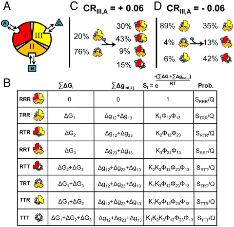
 ) plus the energy of breaking the interactions between domains (
 ). Note: For presentation purposes only, the T states for each domain are depicted as being disordered. In reality, both T and R can be folded and competent to bind ligand. The only requirement is that one of those states (by convention, R) binds ligand with higher affinity. (C) A specific case demonstrating an agonistic allosteric response. Shown are microstates that are significantly populated (i.e., > 3%) before (Left) and after (Right) the addition of ligand A. In the absence of ligand A, the summed probability of microstates with domain III in the R state (i.e., the active microstates—domain III colored yellow) are only marginally populated (approximately 20%). Upon addition of ligand A, redistribution of the ensemble results in a positive shift in the population of these microstates (approximately 73% = 43%+30%), which corresponds to an agonistic response (i.e.,CRIII,A = +0.06). The parameters used are ΔG1 = -1.7, ΔG2 = 2.0, ΔG3 = -0.9, Δg12 = -2.3, Δg23 = 0.1, Δg13 = 1.5, and ΔgLig,A = -5.0 all in kcal/mol. (D) A specific case demonstrating an antagonistic allosteric response. Unlike the case of agonism, the active microstates are significantly populated in the absence of ligand A (approximately 95% = 89%+6%). Upon addition of ligand A, redistribution of the ensemble results in a negative shift in the population of these microstates (35%), which corresponds to an antagonistic response (i.e.,CRIII,A = -0.06). The parameters used are ΔG1 = -2.1, ΔG2 = 1.0, ΔG3 = 1.2, Δg12 = -1.7, Δg23 = 0.6, Δg13 = -2.7, and ΔgLig,A = -5.0, all in kcal/mol.
References
-
- Wright PE, Dyson JH. Intrinsically unstructured proteins: Re-assessing the protein structure-function paradigm. J Mol Biol. 1999;293:321–331. - PubMed
-
- Uversky VU, Oldfiend CJ, Dunker AK. Showing your ID: intrinsic disorder as an Id for recognition, regulation and cell signaling. J Mol Recognit. 2005;18:343–384. - PubMed
-
- Dunker AK, et al. Intrinsically disordered protein. J Mol Graph Model. 2001;19:26–59. - PubMed
-
- Babu MM, Lee R, de Groot NS, Gsponer J. Intrinsically disordered proteins: Regulation and disease. Curr Opin Struc Biol. 2011;21:432–440. - PubMed
Publication types
MeSH terms
Substances
Grants and funding
LinkOut - more resources
Full Text Sources
Other Literature Sources
