Free-energy and illusions: the cornsweet effect

Abstract

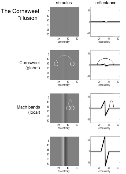
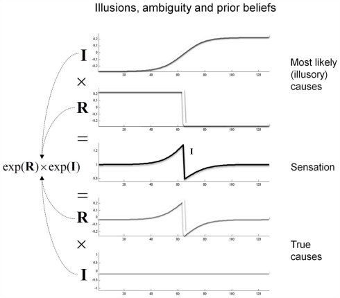
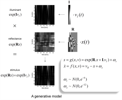
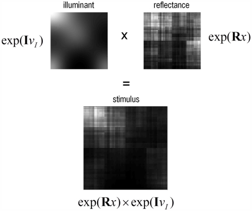
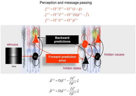
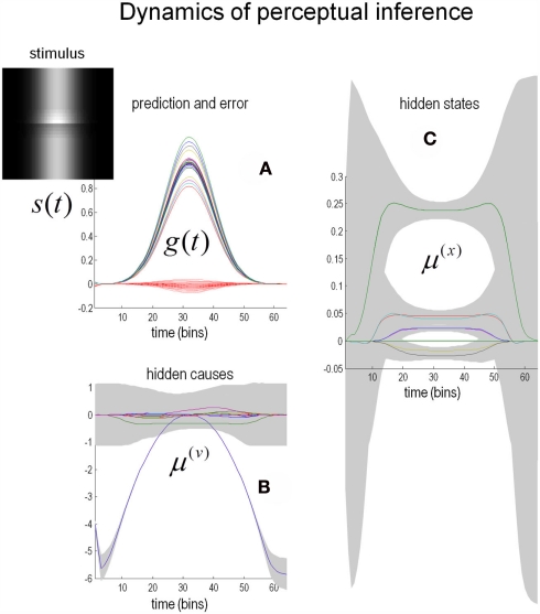
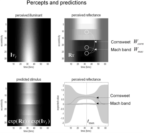
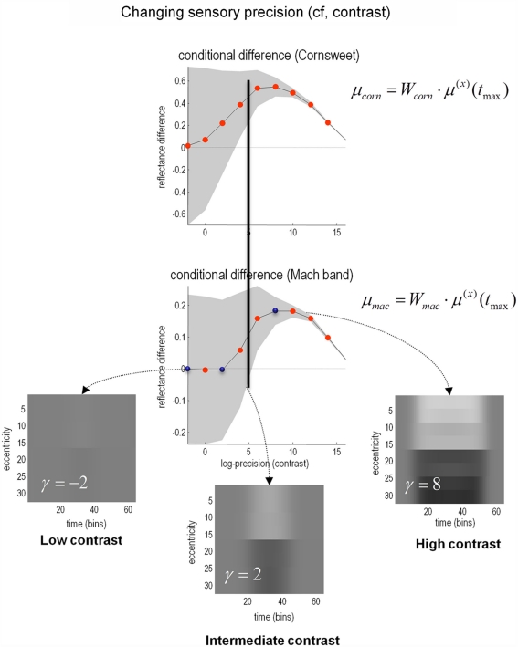
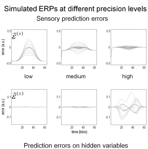
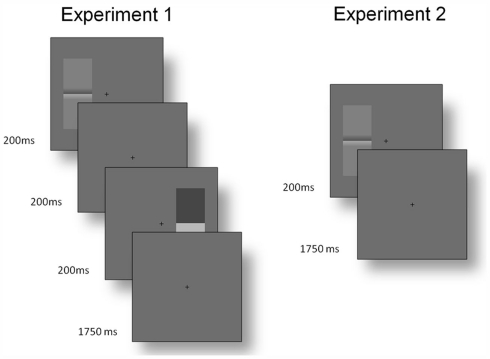
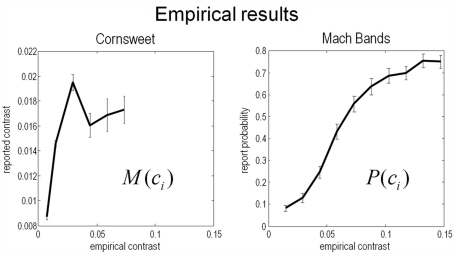
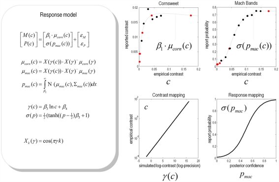
In this paper, we review the nature of illusions using the free-energy formulation of Bayesian perception. We reiterate the notion that illusory percepts are, in fact, Bayes-optimal and represent the most likely explanation for ambiguous sensory input. This point is illustrated using perhaps the simplest of visual illusions; namely, the Cornsweet effect. By using plausible prior beliefs about the spatial gradients of illuminance and reflectance in visual scenes, we show that the Cornsweet effect emerges as a natural consequence of Bayes-optimal perception. Furthermore, we were able to simulate the appearance of secondary illusory percepts (Mach bands) as a function of stimulus contrast. The contrast-dependent emergence of the Cornsweet effect and subsequent appearance of Mach bands were simulated using a simple but plausible generative model. Because our generative model was inverted using a neurobiologically plausible scheme, we could use the inversion as a simulation of neuronal processing and implicit inference. Finally, we were able to verify the qualitative and quantitative predictions of this Bayes-optimal simulation psychophysically, using stimuli presented briefly to normal subjects at different contrast levels, in the context of a fixed alternative forced choice paradigm.

Keywords: Bayesian inference; Cornsweet effect; free-energy; illusions; perception; perceptual priors.

Figure 1

The Cornsweet illusion and Mach bands. The Cornsweet illusion is the false perception that the peripheral regions of a Cornsweet stimulus have different reflectance values. The magnitude of the effect increases as the contrast of the stimulus increases. At higher levels of contrast, the secondary illusion – Mach bands – appear. The Mach bands are situated at the point of inflection of the luminance gradient.

Figure 2

Contributions to luminance. Luminance values reaching the retina are modeled as a multiplication of illuminance from light sources and reflectance from the surfaces in the environment. The factorization of luminance is thus an ill-posed problem. One toy example of this degeneracy is shown here; the same stimulus can be produced by (at least) two possible combinations of illuminance and reflectance. Prior beliefs about the likelihood of these causes can be used to pick the most likely percept.

Figure 3

The generative model: the generative model employed in this paper models illuminance as a discrete cosine function and reflectance as a Harr wavelet function with peripheral high frequency wavelets removed. In addition, illumination is allowed to change quickly over time, whereas reflectance varies more slowly. This is achieved by making the coefficients on the reflectance basis functions hidden states, which accumulate hidden causes to generate changes in reflectance. Inversion of the model provides conditional estimates of the hidden causes and states responsible for sensory input as a function of time. See main text for an explanation of the variables in this figure.

Figure 4

Two-dimension example. The top panels show 2-D examples of luminance (left) and reflectance (right), created form the generative model. The resulting stimulus is the product of the two (bottom panel).

Figure 5

Hierarchical message-passing in the brain. The schematic details a neuronal architecture that optimizes the conditional expectations of hidden variables in hierarchical models of sensory input of the sort illustrated in Figure 3. It shows the putative cells of origin of forward driving connections that convey prediction error from a lower area to a higher area (red arrows) and non-linear backward connections (black arrows) that construct predictions (Mumford, ; Friston, 2008). These predictions try to explain away (inhibit) prediction error in lower levels. In this scheme, the sources of forward and backward connections are superficial and deep pyramidal cells (triangles) respectively, where state-units are black and error-units are red. The equations represent a generalized gradient descent on free-energy (see main text) using the generative model of the previous figure. If we assume that synaptic activity encodes the conditional expectation of states, then recognition can be formulated as a gradient descent on free-energy. Under Gaussian assumptions, these recognition dynamics can be expressed compactly in terms of precision weighted prediction errors: ξ⁽ⁱ⁾:i = s, x, v on the sensory input, motion of hidden states, and the hidden causes. The ensuing equations suggest two neuronal populations that exchange messages; with state-units encoding conditional predictions and error-units encoding prediction error. Under hierarchical models, error-units receive messages from the state-units in the same level and the level above; whereas state-units are driven by error-units in the same level and the level below. These provide bottom-up messages that drive conditional expectations μ⁽ⁱ⁾:i = x, v toward better predictions to explain away prediction error. These top-down predictions correspond to $\tilde{g}:=\tilde{g}\left({\tilde{\mu }}^{\left(x\right)},{\tilde{\mu }}^{\left(v\right)}\right)$ that are specified by the generative model. This scheme suggests the only connections that link levels are forward connections conveying prediction error to state-units and reciprocal backward connections that mediate predictions. Note that the prediction errors that are passed forward are weighted by their precisions: Π⁽ⁱ⁾:i = s, x, v. Technically, this corresponds to generalized predictive coding because it is a function of generalized variables, which are denoted by a (∼), such that every variable is represented in generalized coordinates of motion: for example: $\tilde{x}=\left(x,x^{\prime },x^{″},\dots \right).$ See Friston (2008) for further details.

Figure 6

Predictions of the model. (C) Shows the estimates of the hidden states (coefficients of the reflectance basis functions) over time. The hidden state controlling the amplitude of the lowest-frequency basis function, which corresponds to the Cornsweet percept, contributes substantially to the overall perception of the stimulus (green line). The estimates for the hidden causes are shown in (B). The gray areas are 90% confidence intervals. (A) Shows predictions (solid lines) of sensory input based on the estimated hidden causes and states and the resulting prediction error (dotted red lines). The insert on the upper left shows the time-dependent luminance profile used in this simulation. Please see main text for further details.

Figure 7

The model’s “perceptions.” The upper panels show the predicted illuminance (left) and reflectance profiles (right), reconstructed from the coefficients of the basis functions estimated from the model inversion shown in the previous figure. An inferred reflectance profile demonstrating the Cornsweet illusion is apparent, but at this level of contrast, Mach bands have not yet appeared. Please see main text further details.

Figure 8

The effect of contrast. In the results presented here the precision of the sensory data was used as a proxy for stimulus contrast. As precision increases, the strength of both the Cornsweet and Mach effects increases until, at very high levels of precision (contrast) the true luminance profile is perceived and the illusory percepts fade. Crucially, the Mach bands appear at higher levels of contrast than the Cornsweet illusion. The inserts in the lower panels show the inferred reflectance is at different levels of contrast (indicated by the blue dots in the lower graph). The prediction errors associated with the processing of stimuli at these three levels are shown in the next figure. Please see main text for further details.

Figure 9

Contrast and prediction error. As stimulus contrast increases, prediction error is redistributed from sensory input to hidden variables. At high levels of precision, sensory information induces prediction errors at higher levels, which in turn explain away prediction error at the sensory level. The higher level prediction errors at high precision reflect increasing confidence that the reflectance is different from the prior expectation of zero. Please see main text for further details.

Figure 10

Time courses of trials. Experiment 1: before the start of each trial, participants fixated a central cross. One Cornsweet and one real luminance step stimulus appeared for 200 ms each, with a 200 ms interval between them. The order of the stimuli, their orientation and the side on which each appeared were randomized (although they were constrained to appear on opposite sides within each trial). Participants then had 1750 ms to report the side on which the stimulus with the greatest contrast had appeared (using the arrow keys of the keyboard). Experiment 2: each trial stared with fixation. A Cornsweet stimulus then appeared for 200 ms with a random orientation to the left or right of fixation. Participants had 1750 ms to report, with the “Y” and “N” keys, if they perceived Mach bands.

Figure 11

experimental results. This figure shows the results of the empirical psychophysical study for the Cornsweet illusion (left panel) and the Mach band illusion (Right panel). Both report the average effect over subjects and the SE (bars). The Cornsweet illusion is measured in terms of the subjective contrast level (quantified in terms of subjective equivalence using psychometric functions). The Mach band illusion is quantified in terms of probability that the illusion is reported to be present. Both results are shown as functions of empirical (Weber) stimulus contrast levels. We have used the same range for both graphs so that the dependency on contrast levels can be compared. The key thing to note here is that the Cornsweet illusion peaks before the Mach band illusion (vertical line).

Figure 12

Predicted and experimental results. Theoretical predictions of the empirical results reported in the previous figure: These predictions are based upon a response model that maps from the conditional expectations and precisions in the simulations to the behavioural responses of subjects. This mapping rests on some unknown parameters or coefficients β_i:i = 1, …, 5 that control the relationship between the simulated γ(c) and empirical contrast levels c used for stimuli and the relationship between the probabilities of reporting a Mach band σ(p_mac(c)) and the conditional probability that it exceeds some threshold p_mac(c) at contrast level c. These relationships form the basis of a response model, whose equations are provided in the left panel (for simplicity, we have omitted the expressions for conditional variance of the Mach band contrast). Given empirical responses for the mean Cornsweet effect M(c) and probability of reporting a Mach band P(c), the coefficients β_i can be estimated under the assumption of additive prediction errors ε. The predicted responses following this estimation are shown in the graphs on the right hand side. The upper panels show the empirical data superimposed upon conditional predictions from the model. The gray lines are the predicted psychometric functions, μ_corn(c) and σ(p_mac(c)). The red dots correspond to the predictions at levels of contrast used in the simulations (as shown in Figure 9), while the black dots correspond to the empirical responses: M(c) and P(c). The lower left panel show the relationship between the empirical and simulated contrast levels (as a semi-log plot of the empirical contrast against the log-precision of sensory noise). The lower right panel shows the relationship between the probability of reporting a Mach band is present and the underlying conditional probability that it is above threshold.

References

1. Alink A., Schwiedrzik C. M., Kohler A., Singer W., Muckli L. (2010). Stimulus predictability reduces responses in primary visual cortex. J. Neurosci. 30, 2960–296610.1523/JNEUROSCI.3730-10.2010 - DOI - PMC - PubMed
1. Anderson E. J., Dakin S. C., Rees G. (2009). Monocular signals in human lateral geniculate nucleus reflect the Craik-Cornsweet-O’Brien effect. J. Vis. 9, 1–1810.1167/9.6.1 - DOI - PubMed
1. Barlow H. B. (1974). Inductive inference, coding, perception, and language. Perception 3, 123–13410.1068/p030123 - DOI - PubMed
1. Burton G. J., Moorhead I. R. (1987). Color and spatial structure in natural scenes. Appl. Opt. 26, 157–17010.1364/AO.26.002637 - DOI - PubMed
1. Carandini M., Heeger D. J. (1994). Summation and division by neurons in primate visual cortex. Science 264, 1333–133610.1126/science.8191289 - DOI - PubMed
LinkOut - more resources