Filtered FCS: species auto- and cross-correlation functions highlight binding and dynamics in biomolecules

Abstract

An analysis method of lifetime, polarization and spectrally filtered fluorescence correlation spectroscopy, referred to as filtered FCS (fFCS), is introduced. It uses, but is not limited to, multiparameter fluorescence detection to differentiate between molecular species with respect to their fluorescence lifetime, polarization and spectral information. Like the recently introduced fluorescence lifetime correlation spectroscopy (FLCS) [Chem. Phys. Lett. 2002, 353, 439-445], fFCS is based on pulsed laser excitation. However, it uses the species-specific polarization and spectrally resolved fluorescence decays to generate filters. We determined the most efficient method to generate global filters taking into account the anisotropy information. Thus, fFCS is able to distinguish species, even if they have very close or the same fluorescence lifetime, given differences in other fluorescence parameters. fFCS can be applied as a tool to compute species-specific auto- (SACF) and cross- correlation (SCCF) functions from a mixture of different species for accurate and quantitative analysis of their concentration, diffusion and kinetic properties. The computed correlation curves are also free from artifacts caused by unspecific background signal. We tested this methodology by simulating the extreme case of ligand-receptor binding processes monitored only by differences in fluorescence anisotropy. Furthermore, we apply fFCS to an experimental single-molecule FRET study of an open-to-closed conformational transition of the protein Syntaxin-1. In conclusion, fFCS and the global analysis of the SACFs and SCCF is a key tool to investigate binding processes and conformational dynamics of biomolecules in a nanosecond-to-millisecond time range as well as to unravel the involved molecular states.

Figure 1

Comparison of SACF obtained by using three possible filter-generation scenarios. The species in the simulated mixture have the same lifetime but different rotational correlation times. Both species have the same brightness Q⁽¹⁾=Q⁽²⁾=150 kHz, and identical diffusion times t_d⁽¹⁾=t_d⁽²⁾=0.25 ms. The number of molecules per species are N⁽¹⁾=0.133, N⁽²⁾=0.266, respectively. Dark counts=0.2 kHz, and scatter (IRF)=2.5 kHz rates were considered. The lifetime of both species is τ_G⁽¹⁾=τ_G⁽²⁾=4.0 ns, and the respective rotational correlation times are ρ⁽¹⁾=0.1 ns, ρ⁽²⁾=0.3 ns. The total simulated experiment duration is 2479 s. The SACF for each species are shown in solid blue and red lines for species 1 and 2 respectively. For comparison the simulated correlation function of each species are shown as dashed lines in dark blue and wine for species 1 and 2. 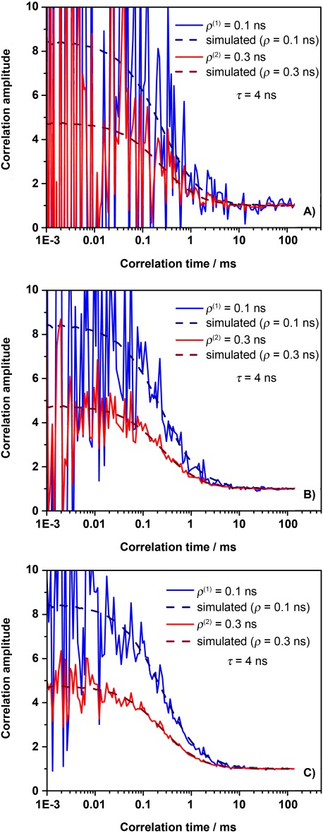A) The calculated SACF by Equation (12) with no split in polarization (scenario 1: assuming as a case imitating single detection channel experiment). The same decay pattern is used for both detection channels and correspondingly the same filters are applied for parallel and perpendicular detection channels to mimic the one detector case. The correlations show poor statistics with some degree of separation between species. B) scenario 2: SACF from Equation (12) using two detectors, independent filter generation for each detection channel and stacking them afterwards. The separation is better compared to the single detector case. C) SACF of scenario 3 using Equation (12) for two detectors and global filter generation. The separation of species is obvious to the eye, and the estimated error in the recovered parameters is within 2 %. A detail error analysis of recovered parameters is done in Section 2.2.

Figure 2

Conditional probabilities of polarization resolved fluorescence decays used in simulations for static and dynamic binding equilibria of two species in buffer: free ligand (ρ^{(free ligand)}=2.71 ns) and complex (ρ^(complex)=5.18 ns).

Figure 3

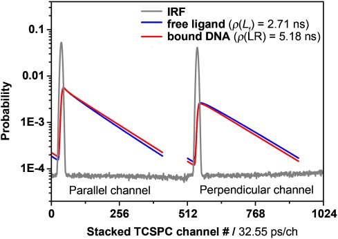
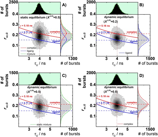
Burstwise analysis of single-molecule events in simulations of an SMD experiment. 2D histograms of fluorescence lifetime (τ_G) distributions on the x axis and scatter-corrected anisotropy r_sc,G on the y axis for mixtures of two species [free-labeled ligand (ρ^{(free ligand)}=2.71 ns) and a complex (ρ^(complex)=5.18 ns)] in buffer. The overlaid red and blue curves show the Perrin equation with a fundamental anisotropy r₀=0.375 and the species-specific rotational correlation times ρ. A) 50 by 50 percent (X^(LR)=0.5) mixture of static species. B) 80 by 20 percent (X^(LR)=0.2) mixture of dynamic species (k_1,2=2000 s⁻¹; k_2,1=8000 s⁻¹ or t_R=0.1 ms), C) 50 by 50 percent (X^(LR)=0.5) mixture of dynamic species (k_1,2=k_2,1=2000 s⁻¹ or t_R=0.25 ms). D) 20 by 80 percent (X^(LR)=0.8) mixture of dynamic species (k_1,2=8000 s⁻¹; k_2,1=2000 s⁻¹ or t_R=0.1 ms). The 1D lifetime τ_G distributions are overlaid by corresponding ones from 50 by 50 percent static mixture (green line). The 1D r_sc,G distributions (gray) are overlaid by distributions from 100 % free ligand (blue line), 50 by 50 percent mixture of static species (green line) and 100 % complex (red line).

Figure 4

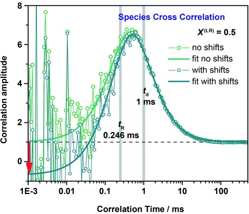
Simulation of an FCS experiment for distinct mixtures of species [free ligand (ρ^{(free Ligand)}=2.71 ns) and complex (ρ^(complex)=5.18 ns)] in buffer with N=0.1. The data generated in the simulation correspond to a measurement time in a real experiment of approximately 12 500 s. The geometric shape of the excitation focus was defined as 3D Gaussian with and . The background signal consists of dark counts=0.2 kHz and scatter=1.8 kHz. The filtered FCS curves were computed by using the filters generated from polarization-resolved decays shown in Figure 2. Comparison of FCCS, SACFs and fit curves for the following cases: A) Overlay of FCCS curves calculated from raw simulated data for 50/50 % static (gray) and 50/50 % dynamic mixtures (green). B) Overlay of SACFs for 50/50 % mixtures: static and dynamic equilibrium, respectively, with (k_1,2=k_2,1=2000 s⁻¹ or t_R=0.25 ms). C) Overlay of SACFs for 20/80 % mixtures: static and dynamic equilibrium, respectively, with (k_1,2=8000 s⁻¹, k_2,1=2000 s⁻¹ or t_R=0.1 ms). D) Overlay of SCCFs for two cases: i) 50/50 % mixtures: static (gray curve) and dynamic (green curve, k_1,2=k_2,1=2000 s⁻¹ or t_R=0.25 ms) equilibrium (fit results to t_R=0.246 ms); ii) 80/20 % mixture in a dynamic equilibrium (pink curve, k_1,2=2000 s⁻¹, k_2,1=8000 s⁻¹ or t_R=0.1 ms). The fit gave t_R=0.096 ms; iii) 20/80 % mixture in a dynamic equilibrium (blue curve, k_1,2=8000 s⁻¹, k_2,1=2000 s⁻¹ or t_R=0.1 ms). The fit results in t_R=0.099 ms.

Figure 5

A) Conditional probabilities of polarization-resolved fluorescence decays used for fFCS. Total brightness Q_tot=400 kHz, τ=4 ns, N=0.1, parameters of the observation volume are as in Section 2.2.1. The details on r(t) are given in the text. B) The species cross correlation functions [data (black circles: t_R=100 μs, open black circles: t_R=10 μs, black squares: t_R=1 μs, open black squares: t_R=0.1 μs), fits by Equation (19) (blue lines)] nicely recover the simulated parameters (magenta).

Figure 6

A) 2D Histogram F_D/F_A versus τ_D(A) of Sx 105/225 labeled with Alexa488 and Alexa594. Grayscale contours represent binned accumulation of single-molecule events with the following parameters: The average green and red background count rates were 〈B_g〉=4.4 kHz, 〈B_r〉=0.39 kHz, respectively. An estimated 4.2 % of cross-talk signal was accounted for. The green over red detection efficiency (g_G/g_R) was 0.8 and the green quantum yield Φ_FD(0)=0.8, red quantum yield Φ_FA=0.4, D-Only lifetime τ_D(0)=4.0 ns, and g-factors 0.995 and 1.378 for green and red channels respectively. On the histogram the main FRET population clearly shows a distribution that is off the static FRET line given by Equation (23) (orange). In dashed green, the dynamic FRET line Equation (24) shows the path taken by the conformational exchange. In this case there are two conformational states, plus a small fraction of D-Only. The open state was identified to have a lifetime τ_D(A)^(open)=3.6 ns and rotational correlation time of ρ=1.5 ns. For the closed state τ_D(A)^(closed)=0.8 ns. B) Conditional probabilities used for generating the filters: buffer (IRF), open [τ_D(A)^(open)=3.6 ns, ρ=1.5 ns] and closed [τ_D(A)^(closed)=0.8 ns, ρ=1.5 ns]. C) Species cross-correlation between closed and open states. Data is fit with Equation (19) and shows a relaxation time of t_R=0.6 ms, and t_d=1.8 ms. On top of this panel, residuals of fit with one or two relaxation times are shown. Additionally, we fit this SCCF globally with SACFs, shown in D), and the fit required two relaxation terms instead of one (t_R1=1.1 ms, t_R2=0.08 ms) with the same t_d=1.8 ms. D) SACFs of the open and closed states as defined by the filters described above. Fits represent the global target fit of the two SACFs and the SCCF. The difference between global target fit of the SACF and SCCF with one and two relaxation times are shown on top of the SACF. The fit requires two relaxation times to reduce the characteristic deviations in the residuals. The SACFs fit with one relaxation time are not shown.

Figure 7

fFCS separates species when difference in rotational correlation time between two species is 0.9 ns whereas the fluorescence lifetimes are the same (4 ns). All other simulation conditions are the same as in Figure 1. The total duration of the simulated experiment is 1598 s. A) Conditional probability of the two species [species 1 ρ⁽¹⁾=0.1 ns in blue and species 2 ρ⁽²⁾=1.0 ns in red]. IRF shape is shown in gray for reference. B) fFCS can separate species. SACF of species 1 and 2 are shown in blue and red respectively. The simulated species are shown as dashed lines for the same case, and represent the expected correlation functions. The noise is significantly reduced from the case presented in Figure 1.

Figure 8

Overlay of SCCFs calculated by fFCS for dynamic mixture of species with X^(LR)=0.5 [free ligand with ρ^{(free ligand)}=2.71 ns and complex with ρ^(complex)=5.18 ns] in buffer without (light green) and with shift (dark green) of species decay curves relative to IRF. Further simulation conditions are given in Figure 3. Shifts of patterns are 0.3 ns and 0.2 ns for the detection channels of parallel and perpendicular polarization, respectively.

Figure 9

Decays and filters for simulated mixture of two species with same fluorescence lifetime but different rotational correlation times. The parameters used for each species in the simulation are Q⁽¹⁾=Q⁽²⁾=150 kHz, t_d⁽¹⁾=t_d⁽²⁾=0.25 ms, N⁽¹⁾=0.133, N⁽²⁾=0.266, dark counts=0.2 kHz, scatter=2.5 kHz. The lifetime of both species is the same (τ_G⁽¹⁾=τ_G⁽²⁾=4.0 ns), and the respective rotational correlation times are ρ⁽¹⁾=0.1 ns, ρ⁽²⁾=0.3 ns. The total duration of the simulated experiment is 2479 s. 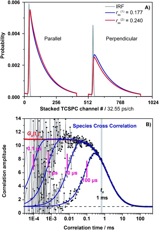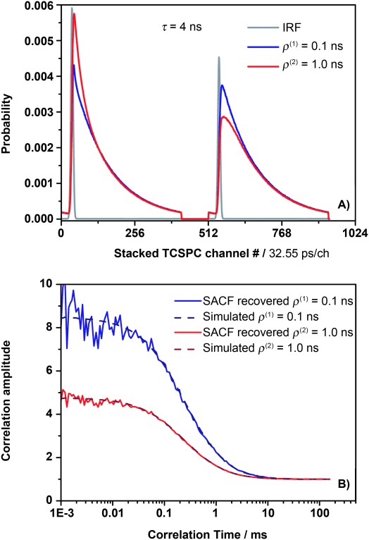A) The normalized TCSPC histograms () for each species as described in Equation (26). The IRF shape is shown in gray. The first species (blue line) has ρ⁽¹⁾=0.1 ns and the second species (red line) has ρ⁽²⁾=0.3 ns. B) The generated filters for each species () are plotted according to the notation: IRF shown in gray, species 1 in blue, and species 2 in red. C) The independently normalized TCSPC histograms for species 1 and 2 according to Equation (27). D) Simultaneously independently minimized filters using Equations (29) and (30). E) Conditional probabilities for each species as described in Equations (4)–(6). The IRF shape is shown in gray. The first species has a rotational correlation of ρ⁽¹⁾=0.1 ns and its decay is shown in blue. The second species with rotational correlation ρ⁽²⁾=0.3 ns is shown in red. F) The filters generated for each species () according to Equations (10) and (11) are plotted. The IRF filter is shown in gray, species 1 in blue, and species 2 in red.

References

-
- Magde D, Elson EL, Webb WW. Phys. Rev. Lett. 1972;29:705–708.
- Rigler R, Foldes-Papp Z, Meyer-Almes FJ, Sammet C, Volcker M, Schnetz A. J. Biotechnol. 1998;63:97–109. - PubMed
Publication types
MeSH terms
Substances
LinkOut - more resources
Full Text Sources