Comparison of list-mode and DIRECT approaches for time-of-flight PET reconstruction

Abstract

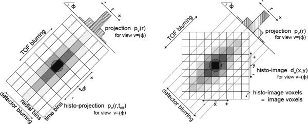
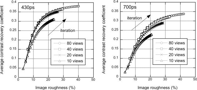
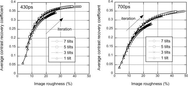
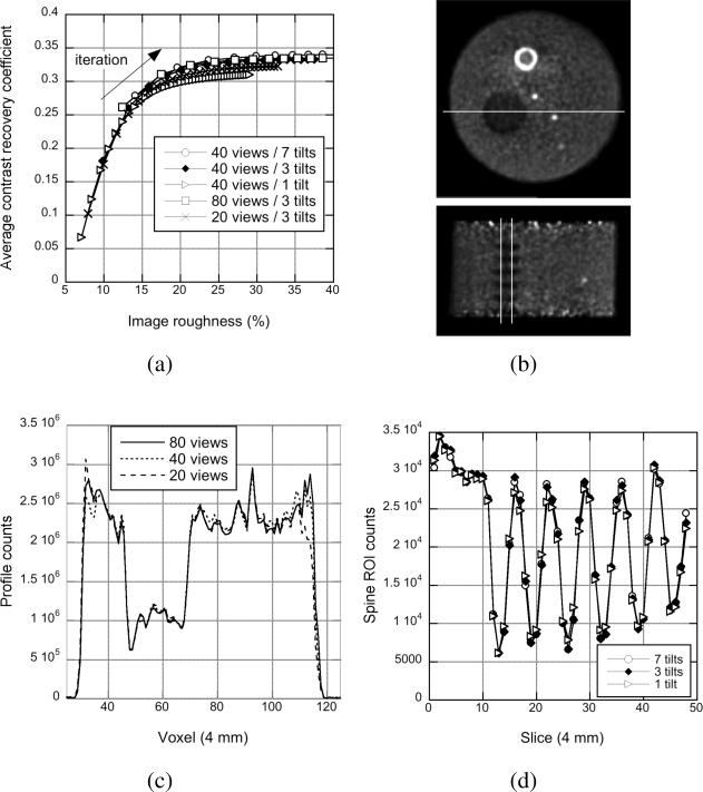
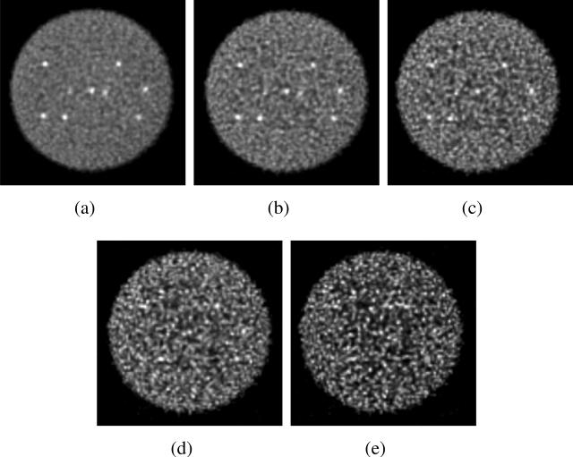
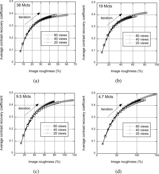
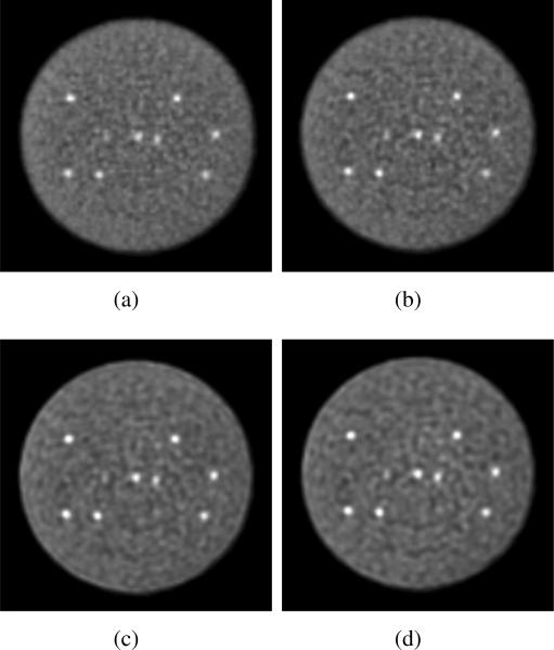
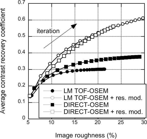
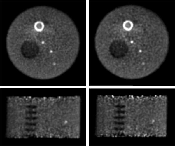
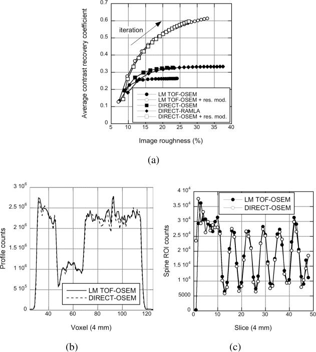
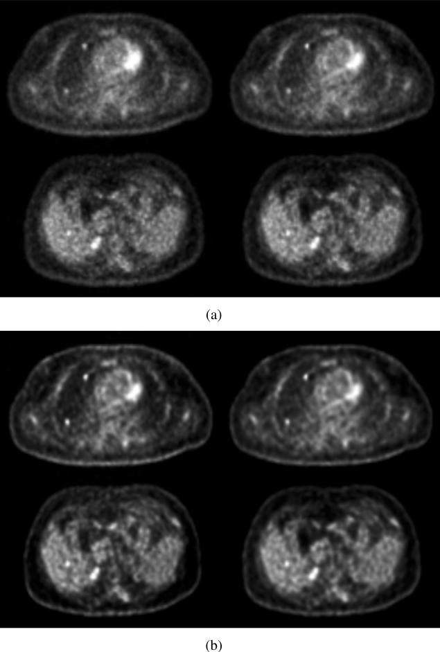
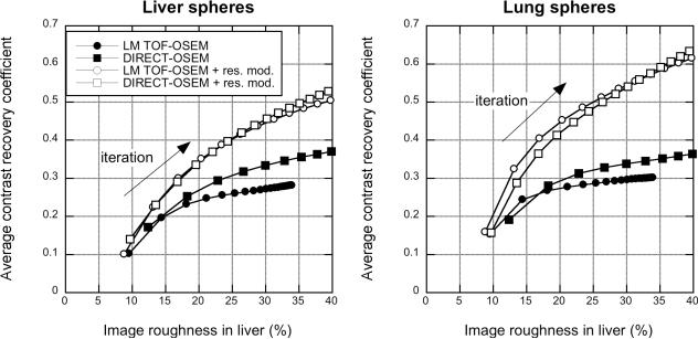
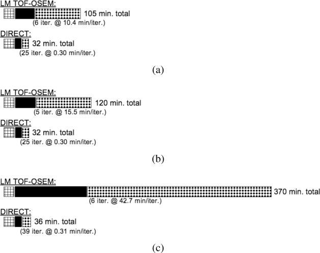
Early clinical results with time-of-flight (TOF) positron emission tomography (PET) systems have demonstrated the advantages of TOF information in PET reconstruction. Reconstruction approaches in TOF-PET systems include list-mode and binned iterative algorithms as well as confidence-weighted analytic methods. List-mode iterative TOF reconstruction retains the resolutions of the data in the spatial and temporal domains without any binning approximations but is computationally intensive. We have developed an approach [DIRECT (direct image reconstruction for TOF)] to speed up TOF-PET reconstruction that takes advantage of the reduced angular sampling requirement of TOF data by grouping list-mode data into a small number of azimuthal views and co-polar tilts and depositing the grouped events into histo-images, arrays with the sampling and geometry of the final image. All physical effects are included in the system model and deposited in the same histo-image structure. Using histo-images allows efficient computation during reconstruction without ray-tracing or interpolation operations. The DIRECT approach was compared with 3-D list-mode TOF ordered subsets expectation maximization (OSEM) reconstruction for phantom and patient data taken on the University of Pennsylvania research LaBr (3) TOF-PET scanner. The total processing and reconstruction time for these studies with DIRECT without attention to code optimization is approximately 25%-30% that of list-mode TOF-OSEM to achieve comparable image quality. Furthermore, the reconstruction time for DIRECT is independent of the number of events and/or sizes of the spatial and TOF kernels, while the time for list-mode TOF-OSEM increases with more events or larger kernels. The DIRECT approach is able to reproduce the image quality of list-mode iterative TOF reconstruction both qualitatively and quantitatively in measured data with a reduced time.

Fig. 1

Comparison of TOF data at a 45° transverse (azimuthal) angle binned into histo-projections (left) and partitioned into histo-images with the DIRECT approach (right). Histo-projections can be thought of as an extension of individual non-TOF projections (radial bins) along the TOF direction (time bins); the sampling intervals relate to the projection geometry and TOF resolution. Histo-images are defined by the geometry and desired sampling (voxel size) of the reconstructed images. For simplicity we illustrate only the 2D case; extension to the 3D case is straightforward: histo-images become 3D voxelized images, and views are defined by both transverse (azimuthal) and co-polar (tilt) angles. The schematics shown represent the deposition of many events from one source location.

Fig. 2

Deposited data from a cylindrical phantom study for three transverse angular views out of 40, showing the effect of gaps between detector modules on histo-images. The data are from the University of Pennsylvania research LaBr₃ TOF-PET system [21], which has 24 detector modules with gaps between modules, each approximately 8 mm, or two crystals, wide. Because of the grouping of angles, gaps do not show up as solid dark bands at regular intervals in the histo-images but as regions of variable, decreased intensity.

Fig. 3

Comparison of image roughness and statistical noise measured using replicate scans in the sphere phantom. Image roughness is plotted as a function of %SD_rep for (a) low and (b) high count densities for list-mode TOF-OSEM and DIRECT-OSEM approaches. (c) Image roughness is plotted as a function of %SD_rep for DIRECT using different numbers of views for the high-count case.

Fig. 4

Horizontal profiles through the local correlation coefficient arrays from the sphere phantom study with 200 M true events. (Left) Pixel correlations are shown for list-mode TOF-OSEM (∘) and DIRECT-OSEM (□) without (closed symbols) and with (open symbols) detector resolution modeling. (Right) Pixel correlations are shown for DIRECT using different numbers of views.

Fig. 5

Sphere phantom: Views - Images of the sphere phantom with 76 M true events as a function of the number of transverse angular views used in DIRECT-RANKA. (Top) Images are shown at 20% image roughness for 430-ps timing resolution data for (from left to right) 80, 40, 20, 10, and 5 views. (Bottom) Images are shown for 700-ps (degraded) timing resolution data.

Fig. 6

Sphere phantom: Views - CRC vs. image roughness performance for the sphere phantom study with 76 M true events as a function of number of transverse angular views used in DIRECT. The average CRC for the 20 spheres is plotted for the data with 430-ps timing resolution (left) and 700-ps (degraded) timing resolution (right) as a function of image roughness for 80 views: ∘, 40 views: □, 20 views: ×, and 10 views: △. The curves were generated for increasing numbers of iterations.

Fig. 7

Sphere phantom: Tilts - Images of the sphere phantom as a function of the number of oblique tilt angles used in DIRECT-RAMLA. (Top) Images are shown at 20% image roughness for the 430-ps timing resolution data for (from left to right) 7, 5, 3, and 1 tilt angles. (Bottom) Images are shown for the 700-ps (degraded) timing resolution data.

Fig. 8

Sphere phantom: Tilts - CRC vs. image roughness performance from the sphere phantom study as a function of the number of oblique tilt angles used in DIRECT. The average CRC for the 20 spheres is plotted for the data with 430-ps timing resolution (left) and 700-ps (degraded) timing resolution (right) as a function of image roughness for 7 tilts: ∘, 5 tilts: □, 3 tilts: ×, and 1 tilt: △.

Fig. 9

Non-uniform phantom: Angular sampling - (a) Average CRC vs. image roughness performance for the three 8-mm diameter hot spheres in the non-uniform phantom shown in (b) for DIRECT with different numbers of transverse views and oblique tilts. (c) Transverse profiles through the lung insert are shown for images with 20% image roughness for DIRECT with 3 tilt angles and 20, 40, and 80 transverse views. (d) Axial profiles through the spine insert are shown for DIRECT with 40 transverse views and 1, 3, and 7 tilt angles.

Fig. 10

Sphere phantom: Statistics - Central transverse images of the sphere phantom with 430-ps TOF resolution for (a) 76 M, (b) 38 M, (c) 19 M, (d) 9.5 M, and (e) 4.7 M true events. The images are shown for 40 angular views and 3 tilts after 40 iterations with DIRECT-RAMLA.

Fig. 11

Sphere phantom: Statistics - CRC vs. image roughness performance for the sphere phantom study with 430-ps TOF resolution for different numbers of true events reconstructed: (a) 38 M, (b) 19 M, (c) 9.5 M, and (d) 4.7 M true events with DIRECT-RAMLA. Each curve was generated for a single count density for increasing numbers of iterations. Results are shown for 3 tilt angles and 80, 40, and 20 views.

Fig. 12

Sphere phantom: Approaches - Transverse images from the sphere phantom study with 430-ps TOF resolution for different reconstruction approaches: (a) list-mode TOF-OSEM, (b) DIRECT-OSEM, (c) list-mode TOFOSEM with spatially invariant detector resolution model, and (d) DIRECT-OSEM and spatially invariant detector resolution model. All images are shown at 15% image roughness.

Fig. 13

Sphere phantom: Approaches - CRC vs. image roughness plots for the sphere phantom study with 430-ps TOF resolution for different reconstruction approaches. Results are shown for list-mode (LM) TOF-OSEM (circles) and DIRECT-OSEM (squares). Results are also shown with a spatially invariant detector resolution model (open symbols).

Fig. 14

Non-uniform phantom - Transverse (top) and coronal (bottom) images of the non-uniform phantom. Images from reconstructions with (left) list-mode TOF-OSEM and (right) DIRECT-OSEM are shown at 20% image roughness. The hot annular structure near the top of the image is a myocardial insert that was not analyzed in this study. The non-uniform background near this insert is most likely due to inaccuracies in the scatter correction. The calculation of image roughness did not include this non-uniform area.

Fig. 15

Non-uniform phantom: Approaches - (a) Average CRC vs. image roughness performance for the three 8-mm diameter hot spheres in the nonuniform phantom study. Results are shown for DIRECT with the OSEM and RAMLA updates and list-mode TOF-OSEM, with and without detector resolution modeling. (b) Transverse profiles through the lung insert and (c) axial profiles through the spine insert are shown for images with 20% image roughness without detector resolution modeling for DIRECT-OSEM with 40 transverse views and 3 tilt angles and for list-mode TOF-OSEM.

Fig. 16

Patient study - Selected transverse slices through lung (top) and liver (bottom) spheres in the patient images. (Left) List-mode TOF-OSEM reconstruction. (Right) DIRECT-OSEM. Images are shown without (a) and with (b) detector resolution modeling. All images are shown at 20% image roughness in the liver. Two lung and one liver spheres are shown.

Fig. 17

Patient study - CRC vs. image roughness plots for the patient study for different reconstruction approaches. Results are shown for CRC averaged over the five liver spheres (left) and six lung spheres (right) for list-mode list-mode TOF-OSEM and DIRECT-OSEM.

Fig. 18

Schematics showing the times for all steps of image reconstruction for list-mode TOF-OSEM (25 subsets) and DIRECT-RAMLA. The data were from the hot sphere phantom study with 164 M prompts (76 M trues). The preprocessing steps (leftmost hatched boxes) include calculations of randoms and scatter estimates; the time to calculate the sensitivity matrix is shown by the solid black boxes. The reconstruction times (rightmost dotted boxes) are for images with 15% image roughness. All times are shown for a single CPU on a Dell Precision T5500 (2.8 GHz with 12 Gb RAM). Total reconstruction times are shown for data with (a) 430-ps timing resolution, (b) 700-ps timing resolution, and (c) 430-ps timing resolution data with a spatially invariant detector resolution model.

References

1. Karp JS, Surti S, Daube-Witherspoon ME, Muehllehner G. Benefit of time-of-flight in PET: Experimental and clinical results. J. Nucl. Med. 2008;49:462–470. - PMC - PubMed
1. Kadrmas DJ, Casey ME, Conti M, Jakoby BW, Lois C, Townsend DW. Impact of time-of-flight on PET tumor detection. J. Nucl. Med. 2009;50:1315–1323. - PMC - PubMed
1. Lois C, Jakoby BW, Long MJ, Hubner KF, Barker DW, Casey ME, et al. An assessment of the impact of incorporating time-of-flight information into clinical PET/CT imaging. J. Nucl. Med. 2010;51:237–245. - PMC - PubMed
1. Snyder DL, Thomas LJ, Jr., Ter-Pogossian MM. A mathematical model for positron-emission tomography systems having time-of-flight measurements. IEEE Trans. Nucl. Sci. 1981;NS-28:3575–3583.
1. Philippe EA, Mullani NA, Wong W-H, Hartz R. Real-time image reconstruction for time-of-flight positron emission tomography (TOFPET) IEEE Trans. Nucl. Sci. 1982;NS-29:524–528.
Publication types