Stochastic population growth in spatially heterogeneous environments

Abstract

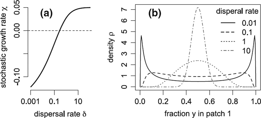
Classical ecological theory predicts that environmental stochasticity increases extinction risk by reducing the average per-capita growth rate of populations. For sedentary populations in a spatially homogeneous yet temporally variable environment, a simple model of population growth is a stochastic differential equation dZ(t) = μZ(t)dt + σZ(t)dW(t), t ≥ 0, where the conditional law of Z(t+Δt)-Z(t) given Z(t) = z has mean and variance approximately z μΔt and z²σ²Δt when the time increment Δt is small. The long-term stochastic growth rate lim(t→∞) t⁻¹ log Z(t) for such a population equals μ − σ²/2 . Most populations, however, experience spatial as well as temporal variability. To understand the interactive effects of environmental stochasticity, spatial heterogeneity, and dispersal on population growth, we study an analogous model X(t) = (X¹(t) , . . . , X(n)(t)), t ≥ 0, for the population abundances in n patches: the conditional law of X(t+Δt) given X(t) = x is such that the conditional mean of X(i)(t+Δt) − X(i)(t) is approximately [x(i)μ(i) + Σ(j) (x(j) D(ji) − x(i) D(i j) )]Δt where μ(i) is the per capita growth rate in the ith patch and D(ij) is the dispersal rate from the ith patch to the jth patch, and the conditional covariance of X(i)(t+Δt)− X(i)(t) and X(j)(t+Δt) − X(j)(t) is approximately x(i)x(j)σ(ij)Δt for some covariance matrix Σ = (σ(ij)). We show for such a spatially extended population that if S(t) = X¹(t)+· · ·+ X(n)(t) denotes the total population abundance, then Y(t) = X(t)/S(t), the vector of patch proportions, converges in law to a random vector Y(∞) as t → ∞, and the stochastic growth rate lim(t→∞) t⁻¹ log S(t) equals the space-time average per-capita growth rate Σ(i)μ(i)E[Y(i)(∞)] experienced by the population minus half of the space-time average temporal variation E[Σ(i,j) σ(i j)Y(i)(∞) Y(j)(∞)] experienced by the population. Using this characterization of the stochastic growth rate, we derive an explicit expression for the stochastic growth rate for populations living in two patches, determine which choices of the dispersal matrix D produce the maximal stochastic growth rate for a freely dispersing population, derive an analytic approximation of the stochastic growth rate for dispersal limited populations, and use group theoretic techniques to approximate the stochastic growth rate for populations living in multi-scale landscapes (e.g. insects on plants in meadows on islands). Our results provide fundamental insights into "ideal free" movement in the face of uncertainty, the persistence of coupled sink populations, the evolution of dispersal rates, and the single large or several small (SLOSS) debate in conservation biology. For example, our analysis implies that even in the absence of density-dependent feedbacks, ideal-free dispersers occupy multiple patches in spatially heterogeneous environments provided environmental fluctuations are sufficiently strong and sufficiently weakly correlated across space. In contrast, for diffusively dispersing populations living in similar environments, intermediate dispersal rates maximize their stochastic growth rate.

Fig. 1

Spatial distribution and population growth in a two patch environment. a The stochastic growth rate χ is plotted as a function of the dispersal rate δ. b The stationary density of the fraction of individuals in patch 1 is plotted for different dispersal rates. Parameter values are μ₁ = μ₂ = 0.3, σ₁ = σ₂ = 1, and D₁₂ = D₂₁ = δ

Fig. 2

The effect of dispersal rate δ on populations emigrating more rapidly out of lower quality patches than higher quality patches. Shown is the stochastic growth rate χ estimated from simulation of the SDE for 100 time units, across a range of values of δ, for both a 40-patch and a 8-patch model. Standard errors are estimated using the standard deviation of the stochastic growth rates across nonoverlapping time segments of a given simulation. Details of the dispersal matrix and parameter values are described in the main text. The right-hand axis shows asymptotic values for δ = 0 and δ = ∞, which are: χ(0) = max_i μ_i and $\chi (\infty )={\mu }^T\pi -\frac{1}{2}{\pi }^T\mathrm{\Sigma }\pi$ (Proposition 2). “High dispersal” shows the approximation of the form χ(δ) ≈ a + b/δ for large δ calculated from formula (19) of Theorem 2

Fig. 3

The effect of dispersal rate δ on populations emigrating more rapidly out of higher quality patches than lower quality patches. Details are as in Fig. 2, but with different dispersal scheme; parameter values are described in the main text

Fig. 4

Effects of spatial correlations on the ideal free patch distribution in a 15 patch environment. Per-capita growth rates μ_i are plotted in the top left. The ideal free patch distribution y* is plotted at three levels of spatial correlation ρ. Covariances are σ_ii = 2 and σ_ij = 2ρ for i ≠ j

References

-
- Adler FR. The effects of averaging on the basic reproduction ratio. Math Biosci. 1992;111:89–98. - PubMed
- Bascompte J, Possingham H, Roughgarden J. Patchy populations in stochastic environments: critical number of patches for persistence. Am Nat. 2002;159:128–137. - PubMed
- Benaïm M, Schreiber SJ. Persistence of structured populations in random environments. Theor Popul Biol. 2009;76:19–34. - PubMed
- Bhattacharya RN. Criteria for recurrence and existence of invariant measures for multidimensional diffusions. Ann Probab. 1978;6(4):541–553. ISSN 00911798. http://www.jstor.org/stable/2243121.
- Bogachev VI, Röckner M, Stannat W. Uniqueness of solutions of elliptic equations and uniqueness of invariant measures of diffusions. Sbornik: Math. 2002;193(7):945. http://stacks.iop.org/1064-5616/193/i=7/a=A01.
Publication types
MeSH terms
Grants and funding
LinkOut - more resources
Full Text Sources
Other Literature Sources
Research Materials