Hierarchy measure for complex networks

Abstract

Nature, technology and society are full of complexity arising from the intricate web of the interactions among the units of the related systems (e.g., proteins, computers, people). Consequently, one of the most successful recent approaches to capturing the fundamental features of the structure and dynamics of complex systems has been the investigation of the networks associated with the above units (nodes) together with their relations (edges). Most complex systems have an inherently hierarchical organization and, correspondingly, the networks behind them also exhibit hierarchical features. Indeed, several papers have been devoted to describing this essential aspect of networks, however, without resulting in a widely accepted, converging concept concerning the quantitative characterization of the level of their hierarchy. Here we develop an approach and propose a quantity (measure) which is simple enough to be widely applicable, reveals a number of universal features of the organization of real-world networks and, as we demonstrate, is capable of capturing the essential features of the structure and the degree of hierarchy in a complex network. The measure we introduce is based on a generalization of the m-reach centrality, which we first extend to directed/partially directed graphs. Then, we define the global reaching centrality (GRC), which is the difference between the maximum and the average value of the generalized reach centralities over the network. We investigate the behavior of the GRC considering both a synthetic model with an adjustable level of hierarchy and real networks. Results for real networks show that our hierarchy measure is related to the controllability of the given system. We also propose a visualization procedure for large complex networks that can be used to obtain an overall qualitative picture about the nature of their hierarchical structure.

Figure 1. An adjustable hierarchical network with the different edge types.

The blue edges belong to the original arborescence graph that is used as the backbone of the adjustable hierarchical (AH) network. There are three type of possible edges added to the graph: down edges (green), horizontal edges (orange) and up edges (red). They have different effects on the hierarchical structure of the directed tree. Down edges conserve the hierarchy, horizontal edges has a slight influence and up edges make strong changes in the structure.

Figure 2. Distribution of the local reaching centrality for the adjustable hierarchical network.

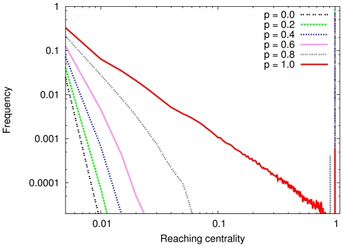
Distribution of the local reaching centrality in the adjustable hierarchical (AH) network model at different parameter values. Each distribution is averaged over 1000 AH networks with and . The standard deviations of the distributions are comparable to the averages only for relative frequencies less than 0.002. Note that from the (highly random) to the (fully hierarchical) state the distribution changes continuously and monotonously with .

Figure 3. The global reaching centrality at different p values in the adjustable hierarchical model.

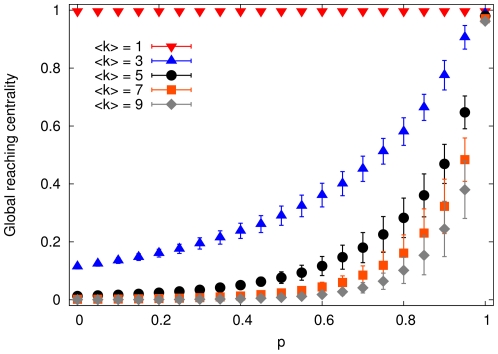
All curves show averages over an ensemble of 1000 networks with and different average degrees. Standard deviations grow with , but they are clearly below the average values of the GRC. Note that for larger density, it is less likely to obtain the same level of hierarchy.

Figure 4. The global reaching centrality versus average degree in the Erdös–Rényi and scale-free networks.

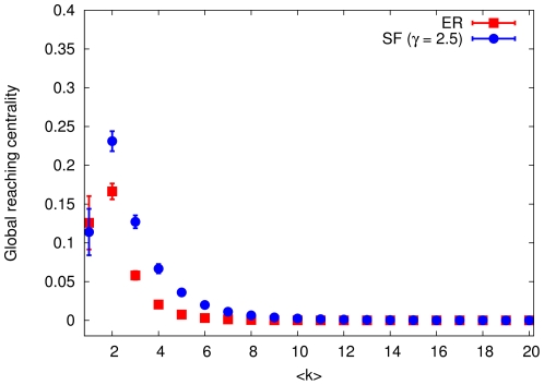
Dots show averages for 1000 graphs with nodes. In the Erdös–Rényi and scale-free networks, standard deviations of the GRC are comparable with its averages only for and , respectively.

Figure 5. Visualization of three network types based on the local reaching centrality.

Visualization of (A) an Erdös–Rényi (ER) network, (B) a scale-free (SF) network and (C) a directed tree with random branching number between 1 and 5. All three graphs have nodes and the ER and SF graphs have . In each network was set to .

Figure 6. Diagram illustrating the process of visualizing an ensemble of networks.

First, we compute the layout based on the selected local quantity for each graph in the ensemble (top right). Next, we separate the levels logarithmically and scale each layout into the unit square (bottom left). Last, we overlay all rescaled layouts and plot the obtained density of nodes in the unit square (bottom right, see color scale also). In the heat maps, the color scale shows , where is the average density of the ensemble.

Figure 7. Visualization of network ensembles.

Visualizations of the (A) Erdös–Rényi, (B) scale-free, (C) directed tree and (D)–(L) AH network ensembles (subfigures (D)–(L) are for different values of the model parameter: ). In each case the color scale shows where is the density averaged over 1000 graphs. and were set. In every network, was set to . The corresponding GRC values are: 0.997 (A), 0.058 (B), 0.127 (C), 0.135 (D), 0.161 (E), 0.194 (F), 0.238 (G), 0.290 (H), 0.361 (I), 0.452 (J), 0.581 (K) and 0.775 (L).

Figure 8. Visualization of real networks.

The hierarchy-based visualization of (A) the GrassLand food web, (B) the electrical circuit benchmark s9234, (C) the transcriptional regulatory network of yeast and (D) the core of the Enron network. In every network was set to .

Figure 9. Distributions of the local reaching centrality for different network types.

For each network type and for the Erdös–Rényi (ER) and scale-free (SF) networks . All curves show averages of the distributions over an ensemble of 1000 graphs. Standard deviations are comparable with the averages only near the peaks in the ER and SF models. Although the standard deviations at the peaks are large, they do not change the positions of the peaks, and thus, do not affect the distributions.

References

-
- Castellano C, Fortunato S, Loreto V. Statistical physics of social dynamics. Phys Rev Lett. 2009;81:591–646.
- Vicsek T, Zafiris A. Collective motion. 2010. arxiv:1010.5017.
- Pastor-Satorras R, Vespignani A. Evolution and Strcuture of the Internet. Cambridge: Cambridge University Press; 2004.
- Albert R, Barabási AL. Statistical Mechanics of Complex Networks. Phys Rev Lett. 2002;74:47–97.
- Pumain D, editor. Hierarchy in Natural and Social Sciences. Dodrecht, The Netherlands: Springer; 2006. pp. 1–12.
Publication types
MeSH terms
Grants and funding
LinkOut - more resources
Full Text Sources
Other Literature Sources