Comparative Study
. 2012 Sep-Dec;106(5-6):239-49.
doi: 10.1016/j.jphysparis.2012.02.001. Epub 2012 Mar 28.

Cortical representation of animate and inanimate objects in complex natural scenes

Affiliations
Comparative Study

Cortical representation of animate and inanimate objects in complex natural scenes

Thomas Naselaris et al. J Physiol Paris. 2012 Sep-Dec.

Abstract

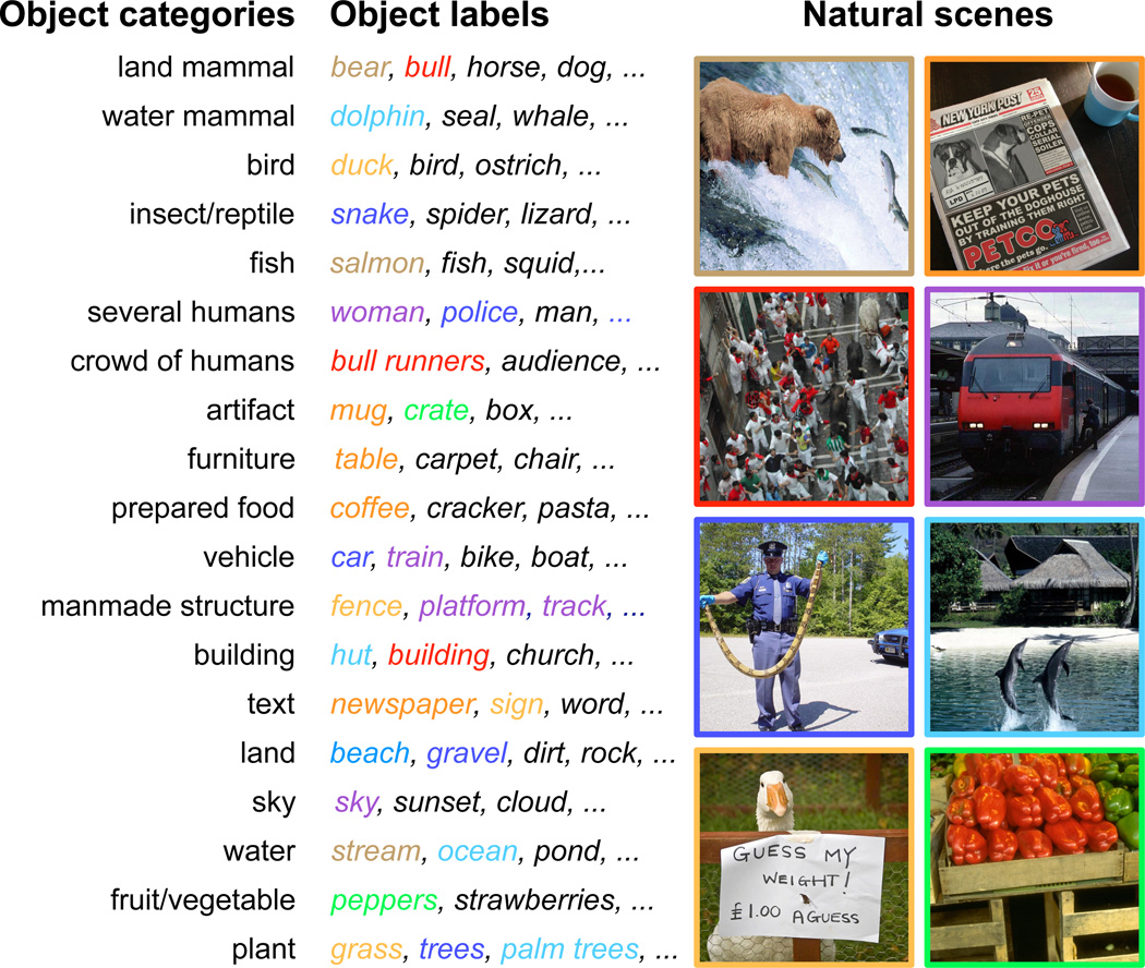
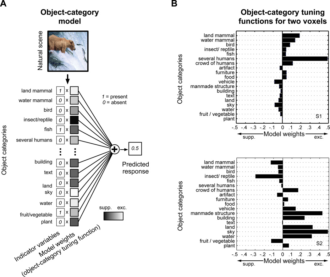
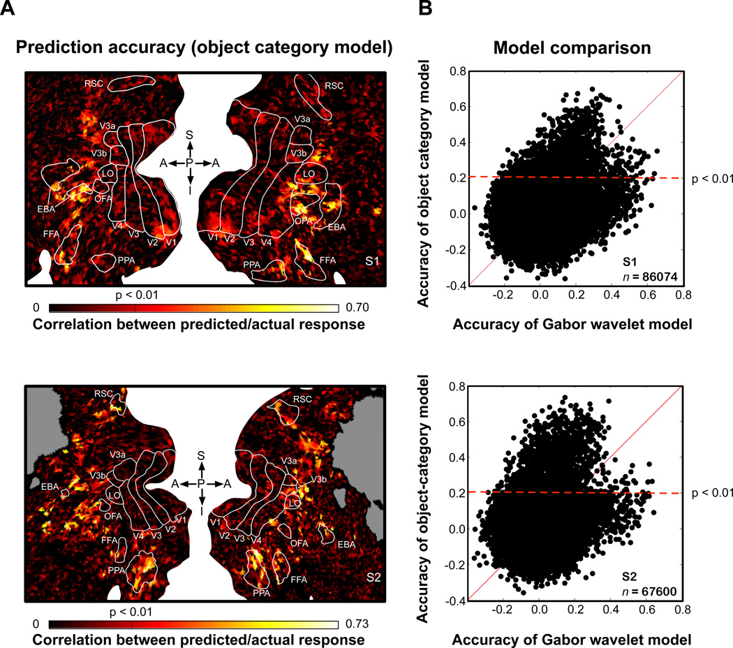
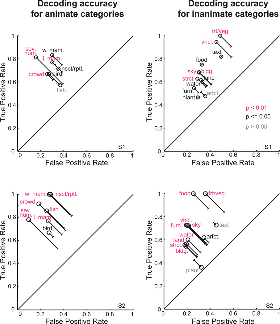
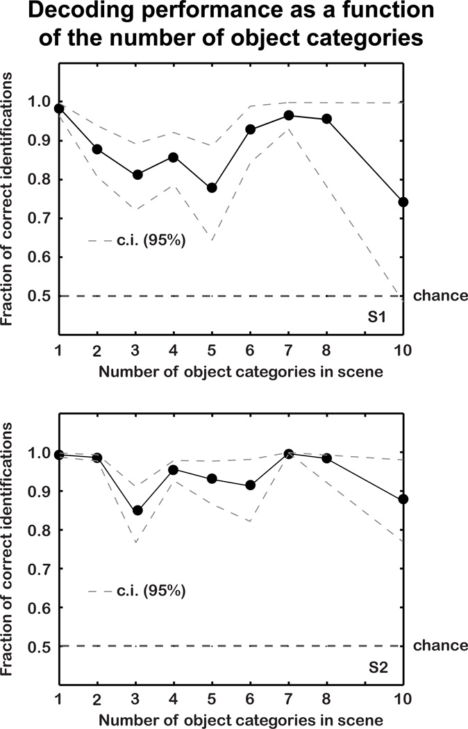
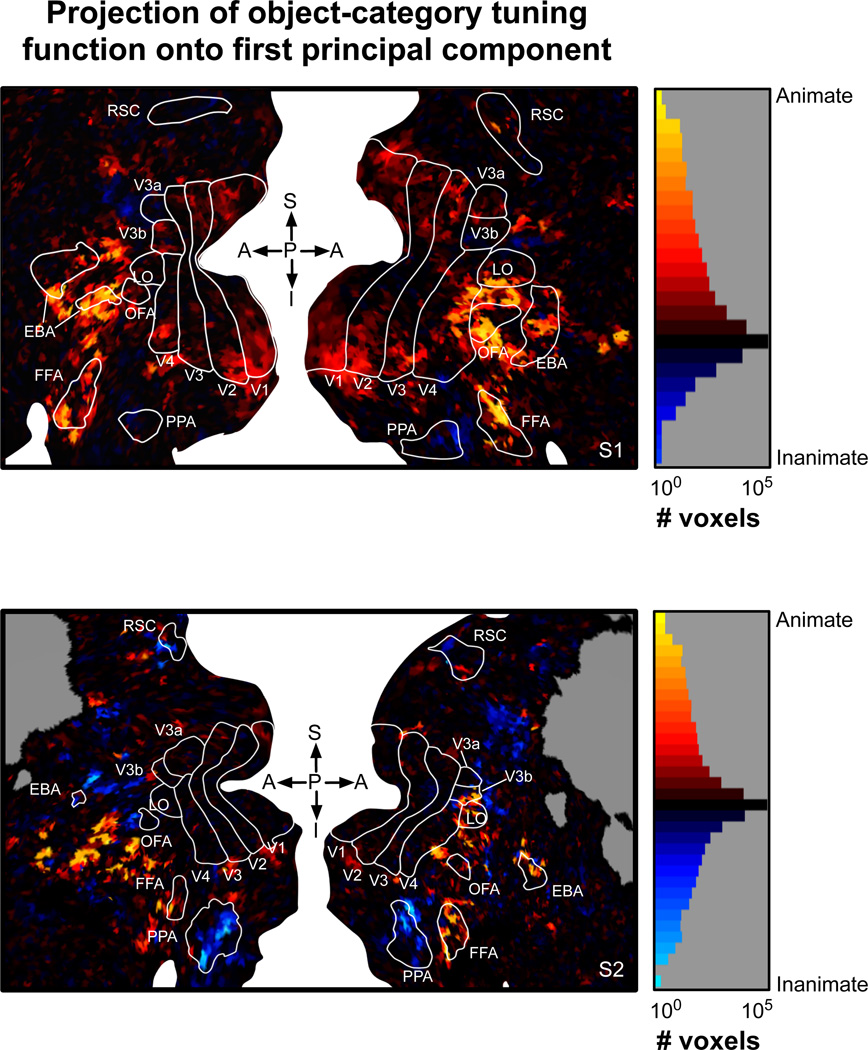
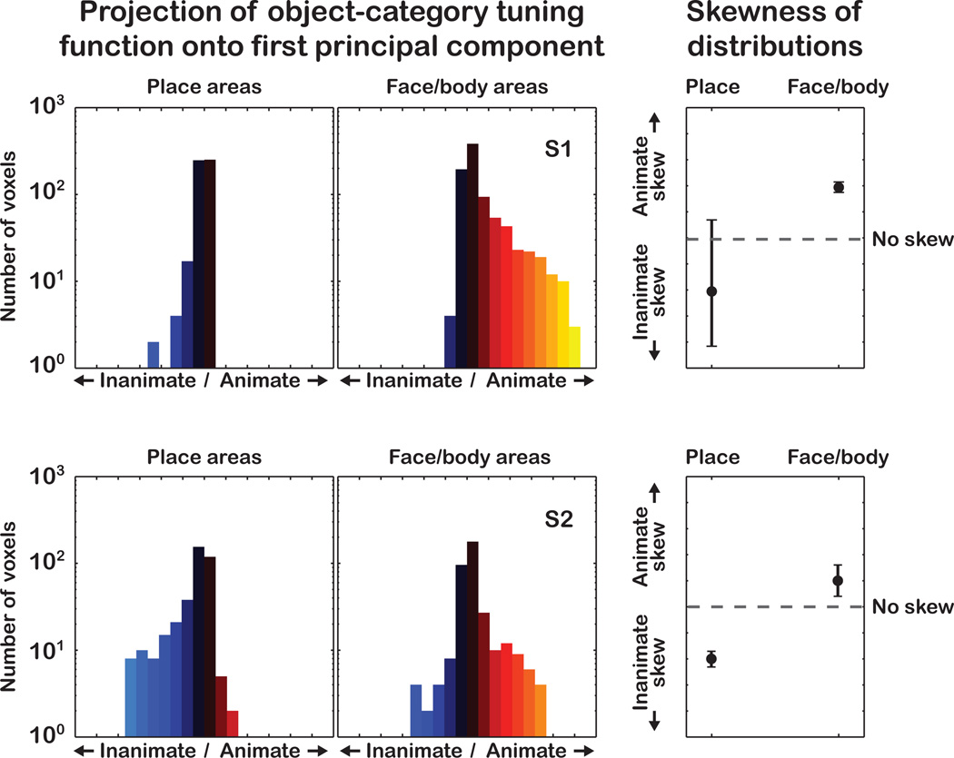
The representations of animate and inanimate objects appear to be anatomically and functionally dissociated in the primate brain. How much of the variation in object-category tuning across cortical locations can be explained in terms of the animate/inanimate distinction? How is the distinction between animate and inanimate reflected in the arrangement of object representations along the cortical surface? To investigate these issues we recorded BOLD activity in visual cortex while subjects viewed streams of natural scenes. We then constructed an explicit model of object-category tuning for each voxel along the cortical surface. We verified that these models accurately predict responses to novel scenes for voxels located in anterior visual areas, and that they can be used to accurately decode multiple objects simultaneously from novel scenes. Finally, we used principal components analysis to characterize the variation in object-category tuning across voxels. Remarkably, we found that the first principal component reflects the distinction between animate and inanimate objects. This dimension accounts for between 50 and 60% of the total variation in object-category tuning across voxels in anterior visual areas. The importance of the animate-inanimate distinction is further reflected in the arrangement of voxels on the cortical surface: voxels that prefer animate objects tend to be located anterior to retinotopic visual areas and are flanked by voxels that prefer inanimate objects. Our explicit model of object-category tuning thus explains the anatomical and functional dissociation of animate and inanimate objects.


Conflict of interest statement

Conflict of Interest:

The authors declare no conflict of interest related to this work.

Figures

Figure 1
Figure 1. Natural scene stimuli labeled with nineteen object categories
(left) A set of nineteen object categories was selected for our analysis of object representation. (middle) A few example objects that are members of each object category. Objects in colored font appear in the corresponding natural scene at far right. (right) All natural scenes shown here were selected from the 1386 presented during the experiment. Prior to the experiment, the objects in each natural scene were labeled and assigned to the appropriate object category. The entire set of natural scenes contained many examples of objects belonging to each category.
Figure 2
Figure 2. An object-category encoding model based on nineteen object categories
(A) A separate object-category model was constructed for each voxel on the cortical surface. The object category model provides a set of positive (excitatory) or negative (suppressive) weights (plotted as shaded squares) that describe how the presence of each category affects measured BOLD activity. Indicator variables pick out the object categories present in the natural scene; the corresponding weights are summed to generate a predicted voxel response. Voxel responses predicted on a separate data set not used to fit the model are used to verify model accuracy. (B) We refer to the set of object-category weights for each voxel as the object-category tuning function. Here the object-category tuning functions for two voxels are plotted as bar charts. The voxel shown at top has the highest prediction accuracy across all voxels for subject 1 (voxel # 21240, prediction accuracy r = 0.697). This voxel is strongly excited by several humans, though land and water mammals also elicit substantial responses. The voxel at bottom has the highest prediction accuracy across all voxels for subject 2 (voxel # 39097, prediction accuracy r = 0.733). This voxel responds to a wide variety of inanimate categories, including sky, water, manmade structures, and buildings. S1 = subject 1. S2 = subject 2.
Figure 3
Figure 3. Prediction accuracy of the object category model
(A) Prediction accuracy of the object-category model was estimated separately for each voxel, and these values were projected onto a cortical flat map (top, subject 1; bottom, subject 2). On the map, white space separates the left and right hemispheres; gray indicates locations outside the slice prescription; white lines demarcate functionally-defined ROIs: V1-V4, primary visual cortical areas; LO, lateral occipical complex; OFA, occipital face area; FFA, fuisform face area; PPA, perihippocampal place area; EBA, extrastriate body area; RSC, retrosplenial cortex. Prediction accuracy is represented using a color scale where black represents low accuracy and yellow represents high accuracy. Prediction accuracy is highest for voxels in visual cortex anterior to highly retinotopic visual areas (i.e., V1-V4). (B) Prediction accuracy for the object-category model compared to prediction accuracy for a Gabor wavelet model. The Gabor wavelet model depends solely on simple visual features (e.g., spatial frequency and orientation) and does not reference the nineteen object categories included in the object-category model. For each voxel, predicted responses to the validation stimuli were generated separately using both the object-category and Gabor wavelet models. Prediction accuracy of the object-category model is plotted on the y-axis, and accuracy of the Gabor wavelet model is plotted on the x-axis. Many voxels (black dots) whose responses are predicted accurately by the object-category model (black dots above the dashed horizontal line) are predicted poorly by the Gabor wavelet model. Thus, the object-category model accurately predicts object-related responses that cannot be explained by simple visual features.
Figure 4
Figure 4. Examples of multiple object categories decoded from complex natural scenes
Decoding can be used to confirm the accuracy of the object-category model. Here the object-category model was used to decode object categories from the responses of voxels for which the object category model provided good predictions (subject 1, n=596; subject 2, n=653). (left) Two natural scene stimuli selected from the validation data set. (right) Object categories that the decoder claims are present in each scene. Object-categories correctly decoded as present (i.e., true positives) are listed in pink, while those incorrectly decoded as present (i.e., false positives) are listed in gray. Decoding is accurate both in heterogeneous scenes that feature objects from many categories (top, subject 1) and in homogeneous scenes that feature objects from fewer categories (bottom, subject 2).
Figure 5
Figure 5. Decoding accuracy for each object category
The object-category model was used to decode the object categories in each image in the validation set, using responses of the same voxels selected in Figure 4. Decoding accuracy for each of the nineteen object categories was analyzed independently. (left) Animate categories. (right) Inanimate categories. (top) Subject 1. (bottom) Subject 2. The vertical axis in each panel gives the true positive rate (TPR), the fraction of scenes in which an object was correctly decoded as present. The horizontal axis in each panel gives the false positive rate (FPR), the fraction incorrectly decoded as present. The solid line at unity represents the TPR and FPR rates that would be expected if the voxel responses provided no decodable information about object category. Object categories farthest from the line at unity are those that were decoded most accurately. Object categories in pink and in black can be decoded significantly (p < 0.01 and p <=0.05 respectively, permutation test). Note that the object categories have different probabilities of occurrence, so the significant distance from line at unity (capped lines indicate significance at p < .05) varies across object category. Most of the animate and inanimate object categories are accurately decoded. Abbreviations: l. mam. = land mammal, w. mam. = water mammal, insct./rptl. = insect/reptile, sev. hum. = several humans, crowd = crowd of humans, arfct. = artifact, furn. = furniture, food = prepared food, vhcl. = vehicle, strct. = manmade structure, bldg. = (part of) building, frt./veg. = fruit/vegetable.
Figure 6
Figure 6. Decoding accuracy as a function of the number of object categories
The horizontal axis gives the number of object categories, and the vertical axis shows the fraction of correct image identifications when the true scene is compared, one-at-a-time, to all other possible scenes. The dashed grey lines indicate bootstrapped 95% confidence intervals. Decoding accuracy shows no systematic relationship to the number of object categories, and the lower bound of the confidence interval is typically above chance (.5) for all numbers of object categories.
Figure 7
Figure 7. Principal component analysis of object tuning functions
Results of principal component (PC) analysis applied to the object-category tuning functions of the same voxels selected in Figures 4 and 5. (left) Coefficients of the first PC are given on the horizontal axis. The coefficients of the first PC are all of the same sign (positive) for animate categories, and are opposite in sign to the most of the coefficients for inanimate categories. The first PC accounts for 50–60% of the variation (y-axis, right panels) in object-tuning functions across voxels (p < .01, permutation test). The significance criterion for each PC (dashed gray line) is the 99th percentile of the histogram of variation explained by the corresponding PC across 10,000 permuted samples. These results suggest that variation in object-category tuning primarily reflects differences in preference for animate and inanimate objects.
Figure 8
Figure 8. Arrangement of animate and inanimate object representations on the cortical surface
(left) A cortical flat map illustrating the projection of each voxel’s object-category tuning function onto the first PC. Details of the maps are the same as in Figure 3. Yellow voxels have large positive projections onto the first PC and generally prefer animate objects. Blue voxels have negative projections onto the first PC and generally prefer inanimate objects. Voxels that prefer animate objects tend to occupy a central density anterior to retinotopic areas. This central density is flanked by voxels with a strong preference for inanimate objects. The locations of these voxels are consistent with the arrangement of category-specific areas (e.g., FFA and PPA), but they extend well beyond the borders of these classical ROIs. (right) Histogram of the projections of object-category tuning functions onto the first PC (log scale). The color scale is matched to the flatmaps at right.
Figure 9
Figure 9. Animate and inanimate object representations in functionally identified regions of interest
(left) Histograms of the projection of the object-tuning functions onto the first PC, for voxels in place-related areas (PPA and RSC) and face or body related areas (FFA, OFA, EBA). (right) Skewness of the histograms with 95% confidence intervals (c.i.). The c.i.'s for skewness were obtained by resampling with replacement the empirical histogram of projection values 10,000 times. The c.i. bounds do not overlap, indicating that place-related areas are skewed toward preference for inanimate categories, and face- and body-related areas are skewed toward preference for animate categories.

Similar articles

Cited by

References

    1. Caramazza A, Shelton JR. Domain-specific knowledge systems in the brain: The animate-inanimate distinction. J. of Cogn. Neurosci. 1998;10:1–34. - PubMed
    1. David SV, Gallant JL. Predicting neuronal responses during natural vision. Network. 2005;16:239–260. - PubMed
    1. Downing PE, Chan AW-Y, Peelen MV, Dodds CM, Kanwisher N. Domain specificity in visual cortex. Cereb. Cortex. 2006;16:1453–1461. - PubMed
    1. Downing PE, Jiang Y, Shuman M, Kanwisher N. A cortical area selective for visual processing of the human body. Science. 2001;293:2470–2473. - PubMed
    1. Epstein R, Kanwisher N. A cortical representation of the local visual environment. Nature. 1998;392:598–601. - PubMed

Publication types

LinkOut - more resources