Pixel-based machine learning in medical imaging

Abstract

Machine learning (ML) plays an important role in the medical imaging field, including medical image analysis and computer-aided diagnosis, because objects such as lesions and organs may not be represented accurately by a simple equation; thus, medical pattern recognition essentially require "learning from examples." One of the most popular uses of ML is classification of objects such as lesions into certain classes (e.g., abnormal or normal, or lesions or nonlesions) based on input features (e.g., contrast and circularity) obtained from segmented object candidates. Recently, pixel/voxel-based ML (PML) emerged in medical image processing/analysis, which use pixel/voxel values in images directly instead of features calculated from segmented objects as input information; thus, feature calculation or segmentation is not required. Because the PML can avoid errors caused by inaccurate feature calculation and segmentation which often occur for subtle or complex objects, the performance of the PML can potentially be higher for such objects than that of common classifiers (i.e., feature-based MLs). In this paper, PMLs are surveyed to make clear (a) classes of PMLs, (b) similarities and differences within (among) different PMLs and those between PMLs and feature-based MLs, (c) advantages and limitations of PMLs, and (d) their applications in medical imaging.

Figure 1

Generalized architecture of an MTANN (a class of PML) consisting of an ML model (e.g., linear-output ANN regression and support vector regression) with subregion input and single-pixel output. All pixel values in a subregion extracted from an input image are entered as input to the ML model. The ML model outputs a single pixel value for each subregion, the location of which corresponds to the center pixel in the subregion. Output pixel value is mapped back to the corresponding pixel in the output image.

Figure 2

Training of an MTANN (a class of PML). An input vector is entered as input to the ML model. An error is calculated by subtracting of a teaching pixel from an output pixel. The parameters such as weights between layers in an ANN model are adjusted so that the error becomes small.

Figure 3

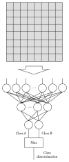
Architecture of a convolution NN (a class of PML). The convolution NN can be considered as a simplified version of the Neocognitron model, which was proposed to simulate the human visual system. The layers in the convolution NN are connected with local shift-invariant inter-connections (or convolution with a local kernel). The input and output of the convolution NN are images and nominal class labels (e.g., Class A and Class B), respectively.

Figure 4

Architecture of a multilayer perceptron for character recognition. The binary pixel values in an image are entered as input to the multilayer perceptron. The class to which the given image belongs is determined as the class of the output unit with the maximum value.

Figure 5

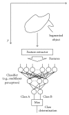
Standard classifier approach to classification of an object (i.e., feature-based ML). Features (e.g., contrast, effective diameter, and circularity) are extracted from a segmented object in an image. Those features are entered as input to a classifier such as a multilayer perceptron. Class determination is made by taking the class of the output unit with the maximum value.

Figure 6

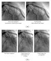
Reduction of quantum noise in angiograms by using a supervised NN filter called a “neural filter.” (a) Images used for training of the neural filter. (b) Result of an application of the trained neural filter to a nontraining image and a comparison result with an averaging filter.

Figure 7

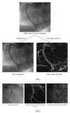
Enhancement of edges from noisy images by use of a supervised edge enhancer called a “neural edge enhancer.” (a) A way to create noisy input images and corresponding “teaching” edge images from noiseless images for training a neural edge enhancer. (b) Result of an application of the trained neural edge enhancer to a nontraining image and a comparison result with a Sobel edge enhancer.

Figure 8

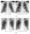
Separation of bones from soft tissue in CXRs by use of an MTANN. (a) Images used for training the MTANN. (b) Result of an application of the trained MTANN to a nontraining CXR.

Figure 9

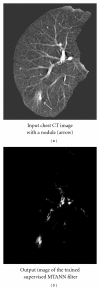
Enhancement of a lesion by use of the trained lesion-enhancement MTANN filter for a nontraining case. (a) Original chest CT image of the segmented lung with a nodule (indicated by an arrow). (b) Output image of the trained lesion-enhancement MTANN filter.

Figure 10

Training of an MTANN for distinction between lesions and non-lesions in a CAD scheme for detection of lesions in medical images. The teaching image for a lesion contains a Gaussian distribution; that for a non-lesion contains zero (completely dark). After the training, the MTANN expects to enhance lesions and suppress non-lesions.

Figure 11

Scoring method for combining pixel-based output responses from the trained MTANN into a single score for each ROI.

Figure 12

Illustrations of various types of nontraining nodules and nonnodules and corresponding output images of the trained MTANN. Nodules are represented by bright pixels, whereas nonnodules are almost dark around the centers of ROIs.

Figure 13

FROC curve indicating the performance of the MTANN in distinction between 57 true positives (nodules) and 1.726 FPs (nonnodules).

References

1. Giger ML, Suzuki K. Computer-aided diagnosis (CAD) In: Feng DD, editor. Biomedical Information Technology. New York, NY, USA: Academic Press; 2007. pp. 359–374.
1. Doi K. Current status and future potential of computer-aided diagnosis in medical imaging. British Journal of Radiology. 2005;78(supplement 1):S3–S19. - PubMed
1. Li F, Sone S, Abe H, MacMahon H, Armato SG, III, Doi K. Lung cancers missed at low-dose helical CT screening in a general population: comparison of clinical, histopathologic, and imaging findings. Radiology. 2002;225(3):673–683. - PubMed
1. Lostumbo A, Wanamaker C, Tsai J, Suzuki K, Dachman AH. Comparison of 2D and 3D views for evaluation of flat lesions in CT colonography. Academic Radiology. 2010;17(1):39–47. - PubMed
1. Soetikno RM, Kaltenbach T, Rouse RV, et al. Prevalence of nonpolypoid (flat and depressed) colorectal neoplasms in asymptomatic and symptomatic adults. Journal of the American Medical Association. 2008;299(9):1027–1035. - PubMed
LinkOut - more resources