Cortical Surface Reconstruction from High-Resolution MR Brain Images

Abstract

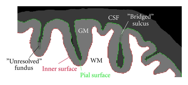
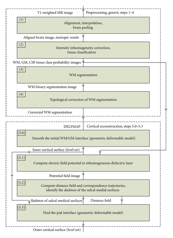
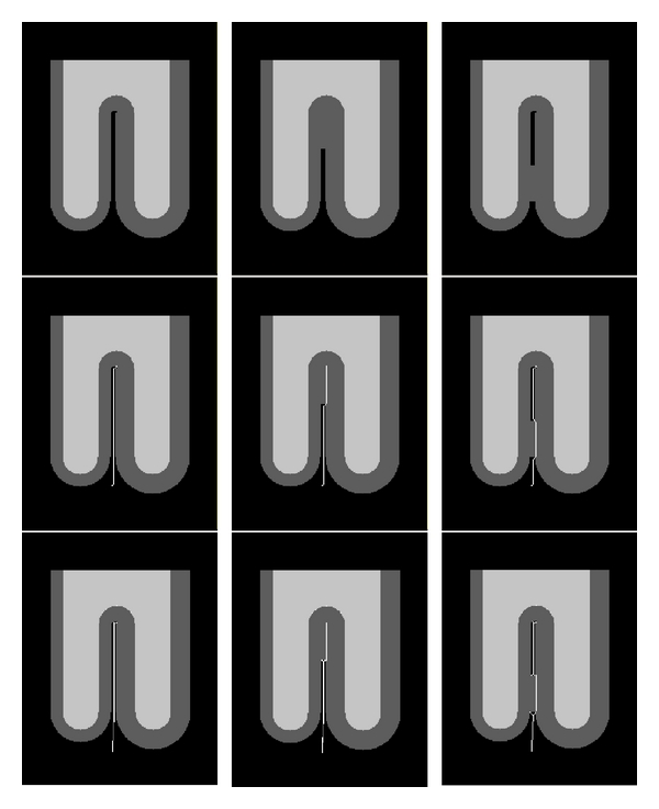
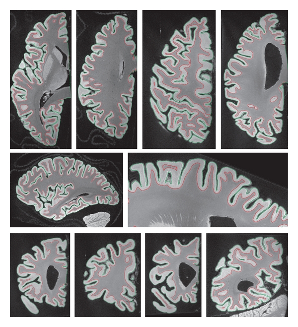
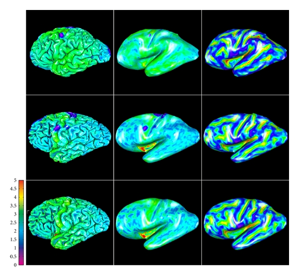
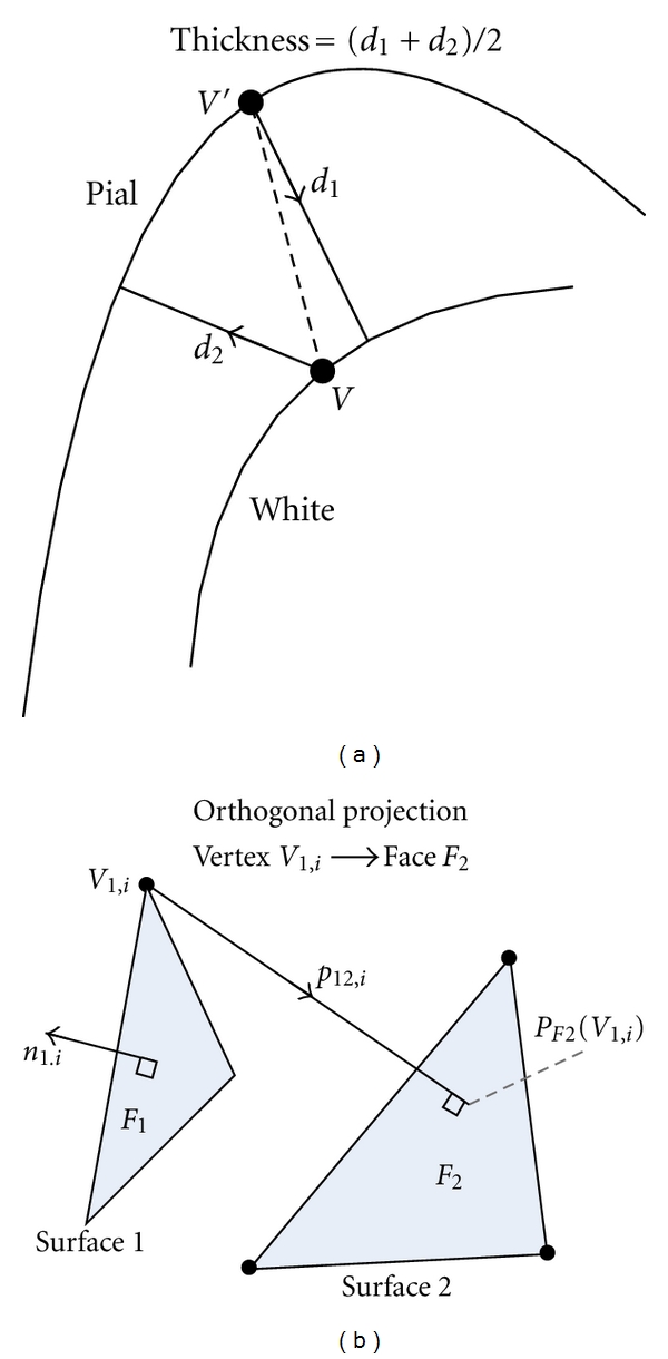
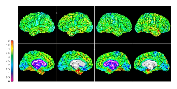
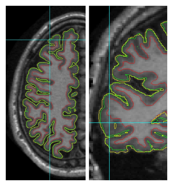
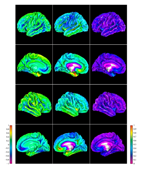
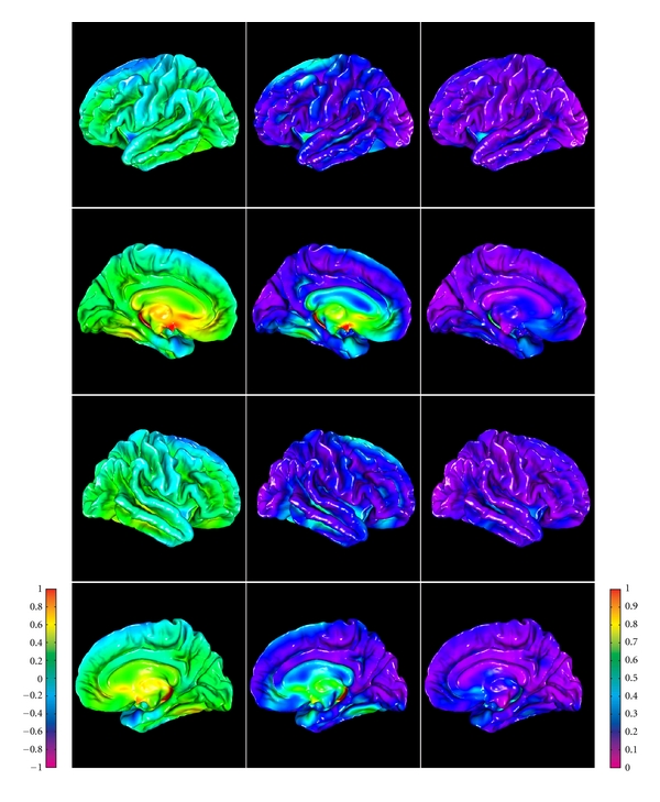
Reconstruction of the cerebral cortex from magnetic resonance (MR) images is an important step in quantitative analysis of the human brain structure, for example, in sulcal morphometry and in studies of cortical thickness. Existing cortical reconstruction approaches are typically optimized for standard resolution (~1 mm) data and are not directly applicable to higher resolution images. A new PDE-based method is presented for the automated cortical reconstruction that is computationally efficient and scales well with grid resolution, and thus is particularly suitable for high-resolution MR images with submillimeter voxel size. The method uses a mathematical model of a field in an inhomogeneous dielectric. This field mapping, similarly to a Laplacian mapping, has nice laminar properties in the cortical layer, and helps to identify the unresolved boundaries between cortical banks in narrow sulci. The pial cortical surface is reconstructed by advection along the field gradient as a geometric deformable model constrained by topology-preserving level set approach. The method's performance is illustrated on exvivo images with 0.25-0.35 mm isotropic voxels. The method is further evaluated by cross-comparison with results of the FreeSurfer software on standard resolution data sets from the OASIS database featuring pairs of repeated scans for 20 healthy young subjects.

Figure 1

Schematic illustration of a fragment of brain slice. Contours of the inner and pial surface are marked in red and green. Due to partial volume effects and limited resolution, adjacent banks of gray matter in some sulci may appear as fused together, creating either a “bridged” sulcus or an unresolved sulcal fundus (a “buried” sulcus). Note that a “bridged” sulcus creates a topological defect, a handle, which may be corrected by a topology-preserving model, whereas a “buried” sulcus does not change the topology.

Figure 2

Block diagram of the overall image processing chain, where the DELFMAP method addresses the reconstruction of cortical surfaces (steps 5.0–5.3) after the preprocessing stage (steps 1–4).

Figure 3

Plots of the stopping/reversal factor β (a) and the distance-constraining factor γ (b) at different values of the “steepness” constant K (solid red line: default K = 40; dashed green line: K = 80; dotted blue line: K = 20).

Figure 4

Cross-sections of simulated test images. (a) The input image; (b) field lines in the uniform permittivity model (Laplace equation). Bottom row: isocontours (c) and field lines (d) in the DELFMAP model with the dielectric layer (dark gray in the input image).

Figure 5

Cross-sections of simulated test images (left: fully resolved sulcus; middle: unresolved fundus; right: bridged sulcus). The white line shows the location of the identified sulcal medial surface skeleton. Comparison of DELFMAP (middle row) versus ACE (bottom row) shows that skeletons produced by DELFMAP have a more regular structure compared to ACE skeletons, which can have small extraneous branches and discontinuities. In the bottom row (ACE), small spurious components are visible at the fundus very close to WM, which in ACE method have to be suppressed by thresholding the distance from WM.

Figure 6

Isocontours of the zero level sets of reconstructed cortical surfaces overlaid on cross-sections of high-resolution MR images (red: the inner surface; green: the outer surface; top, middle, and bottom rows: examples of axial, sagittal, and coronal sections (not to scale), resp.).

Figure 7

Lateral view of pial surfaces from three high-resolution datasets (left column: thickness maps; middle column: inflated thickness maps; right column: inflated convexity maps).

Figure 8

Illustration of two different approaches of defining a distance between two surface meshes. (a) The thickness measure defined in FreeSurfer (2D schematic drawing). (b) The (signed) distance measure defined by closest orthogonal projection.

Figure 9

Example of side-by-side comparison of DELFMAP (column 1 and 3) and FreeSurfer (column 2 and 4) thickness maps (OAS1_202_1, on pial surfaces, left/right hemisphere in the left/right two columns, resp.; 1st row: lateral surface; 2nd row: medial surface; colorbar range 0–5 mm).

Figure 10

Contours of reconstructed cortical surfaces overlaid on the axial (left) and coronal (right) slice (red: inner surface; green: DELFMAP pial surface; yellow: FreeSurfer pial surface; note that the yellow contour appears jagged because it is displayed from FreeSurfer's volumetric signed distance function sampled at 1 mm grid, whereas red and green contours are from level set functions sampled at a finer resolution; left and right images are not to scale). On the left image at the cross-line cursor position (superior frontal region), the yellow contour of FreeSurfer's pial reconstruction oversegments into meningeal space, and a similar trend is noticeable next to cursor on the right image (temporal region).

Figure 11

Group-average maps of intermethod (DELFMAP-FreeSurfer) geometric differences in pial surface reconstructions, resampled to FreeSurfer's average template (left column: signed distance mean, colorbar range ±1 mm, negative/positive values mean FreeSurfer' surface is inside/outside of DELFMAP' surface, resp.; middle column: absolute distance mean, colorbar range 0-1 mm; right column: absolute distance stdev., colorbar range 0-1 mm; rows 1–4: lateral/medial surface of left/right hemisphere, resp.).

Figure 12

Group-average maps of intermethod (DELFMAP-Freesurfer) cortical thickness differences, resampled to FreeSurfer's average template (left column: signed difference mean, colorbar range ±1 mm, negative/positive values mean thickness measured with DELFMAP is smaller/larger than measured with FreeSurfer, resp.; middle column: absolute difference mean, colorbar range 0-1 mm; right column: absolute difference stdev., colorbar range 0-1 mm; rows 1–4: lateral/medial surface of left/right hemisphere, resp.).

Algorithm 1

The level set function update algorithm.

References

1. Han X, Pham DL, Tosun D, Rettmann ME, Xu C, Prince JL. CRUISE: cortical reconstruction using implicit surface evolution. NeuroImage. 2004;23(3):997–1012. - PubMed
1. Kim JS, Singh V, Lee JK, et al. Automated 3-D extraction and evaluation of the inner and outer cortical surfaces using a Laplacian map and partial volume effect classification. NeuroImage. 2005;27(1):210–221. - PubMed
1. Dale AM, Fischl B, Sereno MI. Cortical surface-based analysis: i. segmentation and surface reconstruction. NeuroImage. 1999;9(2):179–194. - PubMed
1. Fischl B, Sereno MI, Dale AM. Cortical surface-based analysis: II. Inflation, flattening, and a surface-based coordinate system. NeuroImage. 1999;9(2):195–207. - PubMed
1. Fischl B, Liu A, Dale A. Automated manifold surgery: constructing geometrically accurate and topologically correct models of the human cerebral cortex. IEEE Transactions on Medical Imaging. 2001;20(1):70–80. - PubMed