. 2013 Jun;35(6):1328-42.
doi: 10.1109/TPAMI.2012.129.

A sparse structure learning algorithm for Gaussian Bayesian Network identification from high-dimensional data

Affiliations

A sparse structure learning algorithm for Gaussian Bayesian Network identification from high-dimensional data

Shuai Huang et al. IEEE Trans Pattern Anal Mach Intell. 2013 Jun.

Abstract

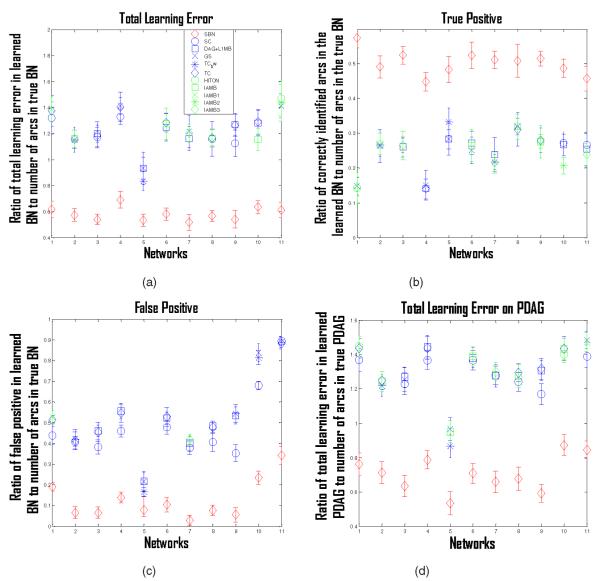
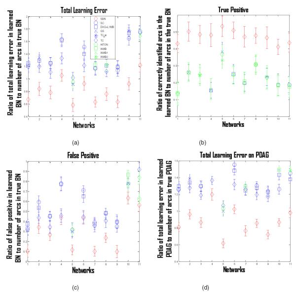
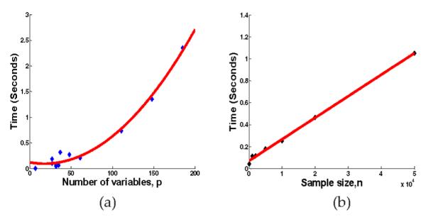
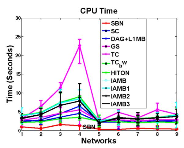
Structure learning of Bayesian Networks (BNs) is an important topic in machine learning. Driven by modern applications in genetics and brain sciences, accurate and efficient learning of large-scale BN structures from high-dimensional data becomes a challenging problem. To tackle this challenge, we propose a Sparse Bayesian Network (SBN) structure learning algorithm that employs a novel formulation involving one L1-norm penalty term to impose sparsity and another penalty term to ensure that the learned BN is a Directed Acyclic Graph--a required property of BNs. Through both theoretical analysis and extensive experiments on 11 moderate and large benchmark networks with various sample sizes, we show that SBN leads to improved learning accuracy, scalability, and efficiency as compared with 10 existing popular BN learning algorithms. We apply SBN to a real-world application of brain connectivity modeling for Alzheimer's disease (AD) and reveal findings that could lead to advancements in AD research.


Figures

Fig. 1
Fig. 1
A Bayesian network structure (DAG).
Fig. 2
Fig. 2
The BCD algorithm used for solving (2).
Fig. 3
Fig. 3
The shooting algorithm used for solving (3).
Fig. 4
Fig. 4
A general tree.
Fig. 5
Fig. 5
A general inverse tree.
Fig. 6
Fig. 6
(a) General tree used in the simulation study in Section 5.1; (b) general inverse tree used in the simulation study in Section 5.2 (regression coefficients of arcs generated from ±Uniform(0.5, 1)).
Fig. 7
Fig. 7
(a) Frequency of X1 being identified as a parent of Xi, i = 2, …, 7; (b) ratio of number of correctly identified arcs in learned BN to number of arcs in true BN; (c) ratio of total learning error in learned BN (false positives plus false negatives) to number of arcs in true BN.
Fig. 8
Fig. 8
(a) Frequency of Xi being identified as parents of their respective child in true BN, i = 1, …, 30; (b) ratio of number of correctly identified arcs in learned BN to number of arcs in true BN; (c) ratio of total learning error in learned BN (false positives plus false negatives) to number of arcs in true BN
Fig. 9
Fig. 9
(a) Ratio of total learning error in the learned BN (false positives plus false negatives) to the number of arcs in the true BN for the 10 competing algorithms and SBN on 11 benchmark networks; (b) ratio of correctly identified arcs in the learned BN (i.e., true positives) to the number of arcs in the true BN; (c) ratio of falsely identified arcs in the learned BN (i.e., false positives) to the number of arcs in the true BN; (d) ratio of the total learning error in the learned PDAG to the number of arcs in the true PDAG. The learned BN and PDAG in (a)-(d) are based on a simulation dataset of sample size 1,000. Dots are means and error bars are standard deviations.
Fig. 10
Fig. 10
(a) Ratio of total learning error in the learned BN (false positives plus false negatives) to the number of arcs in the true BN for the 10 competing algorithms and SBN on 11 benchmark networks; (b) ratio of correctly identified arcs in the learned BN (i.e., true positives) to the number of arcs in the true BN; (c) ratio of falsely identified arcs in the learned BN (i.e., false positives) to the number of arcs in the true BN; (d) ratio of the total learning error in the learned PDAG to the number of arcs in the true PDAG. The learned BN and PDAG in (a)-(d) are based on a simulation dataset of sample size 100. Dots are means and error bars are standard deviations.
Fig. 11
Fig. 11
Scalability of SBN with respect to (a) the number of variables, p, (b) the sample size, n.
Fig. 12
Fig. 12
Comparison of SBN with competing algorithms on CPU time in structure learning. Y -axis is the CPU time for each sweep through all the columns of B on a computer with Intel Core 2, 2.2 GHz, 4 GB memory. The X-axis is the first nine networks in Table 1.
Fig. 13
Fig. 13
Brain effective connectivity models by SBN. (a) AD; (b) NC.

References

    1. Friedman N, Linial M, Nachman I, Péer D. Using Bayesian Networks to Analyze Expression Data. J. Computational Biology. 2000;vol. 7:601–620. - PubMed
    1. Rodin AS, Boerwinkle E. Mining Genetic Epidemiology Data with Bayesian Networks I: Bayesian Networks and Example Application (Plasma apoE Levels) Bioinformatics. 2005;vol. 21(no. 15):3273–3278. - PMC - PubMed
    1. Marcot BG, Holthausen RS, Raphael MG, Rowland M, Wisdom M. Using Bayesian Belief Networks to Evaluate Fish and Wildlife Population Viability under Land Management Alternatives from an Environmental Impact Statement. Forest Ecology and Management. 2001;vol. 153(nos. 1-3):29–42.
    1. Borsuk ME, Stow CA, Reckhow KH. A Bayesian Network of Eutrophication Models for Synthesis, Prediction, and Uncertainty Analysis. Ecological Modelling. 2004;vol. 173:219–239.
    1. Dai H, Korb KB, Wallace CS, Wu X. A Study of Casual Discovery with Weak Links and Small Samples. Proc. 15th Int’l Joint Conf. Artificial Intelligence.1997. pp. 1304–1309.

Publication types