A-current and type I/type II transition determine collective spiking from common input

Abstract

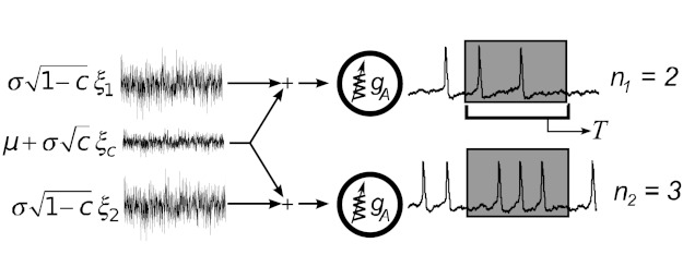
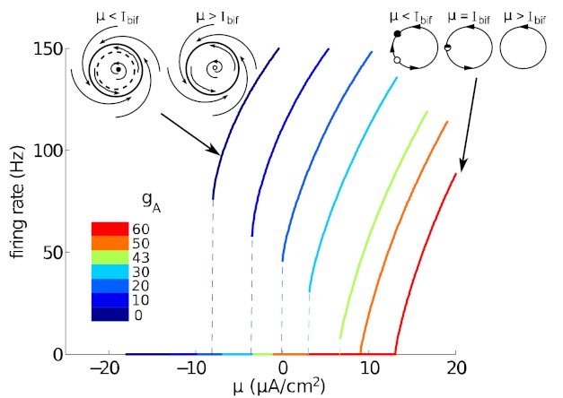
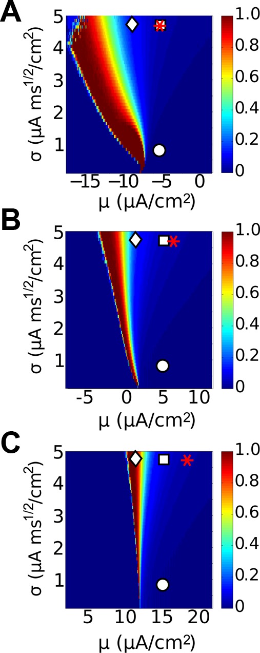
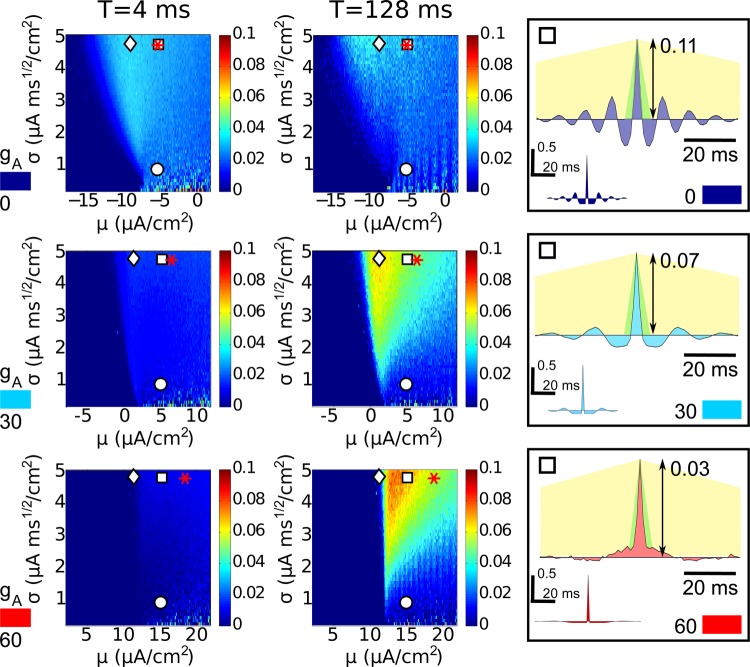
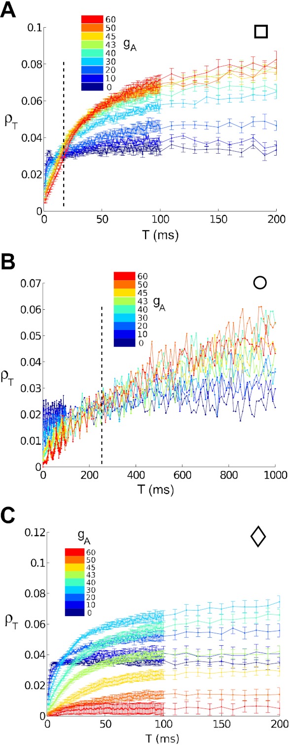
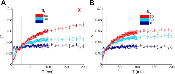
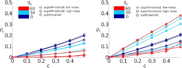
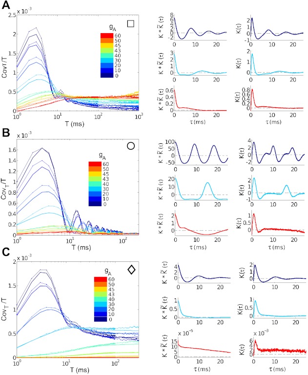
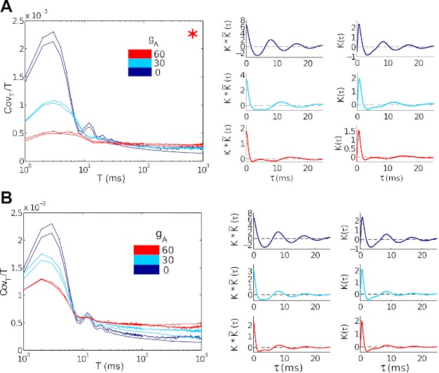
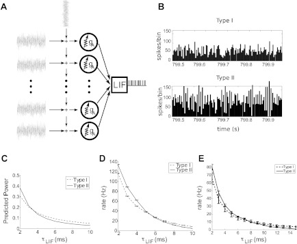
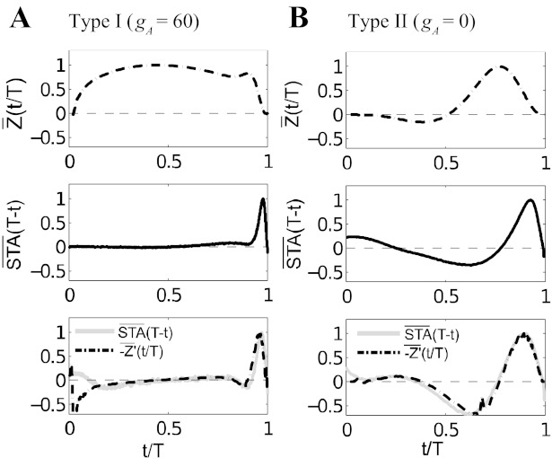
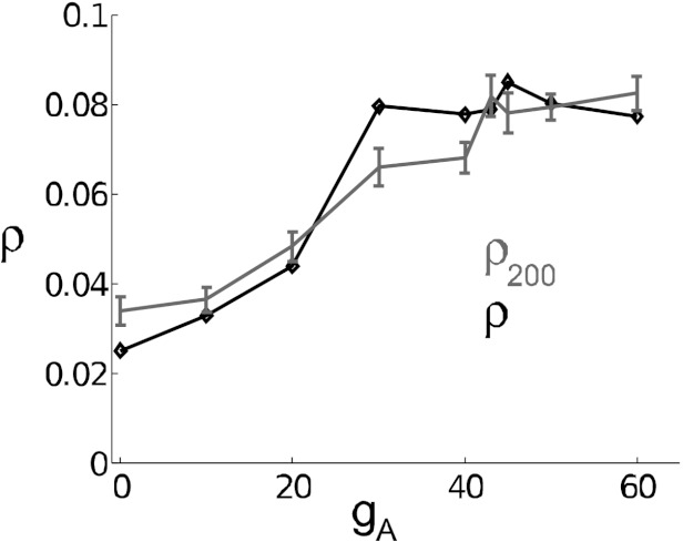
The mechanisms and impact of correlated, or synchronous, firing among pairs and groups of neurons are under intense investigation throughout the nervous system. A ubiquitous circuit feature that can give rise to such correlations consists of overlapping, or common, inputs to pairs and populations of cells, leading to common spike train responses. Here, we use computational tools to study how the transfer of common input currents into common spike outputs is modulated by the physiology of the recipient cells. We focus on a key conductance, g(A), for the A-type potassium current, which drives neurons between "type II" excitability (low g(A)), and "type I" excitability (high g(A)). Regardless of g(A), cells transform common input fluctuations into a tendency to spike nearly simultaneously. However, this process is more pronounced at low g(A) values. Thus, for a given level of common input, type II neurons produce spikes that are relatively more correlated over short time scales. Over long time scales, the trend reverses, with type II neurons producing relatively less correlated spike trains. This is because these cells' increased tendency for simultaneous spiking is balanced by an anticorrelation of spikes at larger time lags. These findings extend and interpret prior findings for phase oscillators to conductance-based neuron models that cover both oscillatory (superthreshold) and subthreshold firing regimes. We demonstrate a novel implication for neural signal processing: downstream cells with long time constants are selectively driven by type I cell populations upstream and those with short time constants by type II cell populations. Our results are established via high-throughput numerical simulations and explained via the cells' filtering properties and nonlinear dynamics.

Fig. 1.

Shared input microcircuit, in which two neurons receive input currents with a common component that represents correlated activity or shared afferents upstream. Each neuron is a single-compartment Connor-Stevens model (see methods), with a maximal A-current conductance g_A that we vary, eliciting a full range of type I to type II spiking dynamics. Shared input currents lead to correlated spikes, which are quantified as shown via spike counts n₁, n₂ over sliding time windows of length T. The input currents received by each cell have mean μ and fluctuate with total variance σ²; the common noise is chosen with variance σ²c and independent noise terms with variance σ²(1 − c).

Fig. 2.

Firing rate vs. injected current (f-I) curves, for the deterministic (σ = 0) Connor- Stevens model. Several values of g_A, yielding a range from type II to type I excitability, are shown; note the nonzero “onset” firing rates and type II excitability for g_A ≈ 0 mS/cm², zero onset rate and type I excitability for g_A ≈ 60 mS/cm², and a gradual transition between. Insets: cartoons of dynamical transitions that lead to nonzero vs. zero onset rates: a subcritical Hopf bifurcation (left) and a saddle-node on invariant circle bifurcation (right); see text for definitions.

Fig. 3.

Fano factor of spike counts over a long time window (T = 256 ms) for a ∼200 × 50 grid of values for the mean current μ and variance σ². From top to bottom, type II to type I: g_A = 0 (A), g_A = 30 (B), and g_A = 60 mS/cm² (C). Markers indicate relative location of (μ, σ)-pair; subthreshold by 1 μA/cm² (diamond), superthreshold by 2 μA/cm² with low noise (circle) and high noise (square), and superthreshold with matched Fano factors (asterisk, see text).

Fig. 4.

Spike count correlations for three models at both short and long time scales. Each row displays data from a value of g_A: from top to bottom, type II (g_A = 0 mS/cm²), intermediate (g_A = 30 mS/cm²), and type I (g_A = 60 mS/cm²). Left: spike count correlations ρ, for short windows T = 4 ms. Middle: spike count correlations ρ_T, for long windows T = 128 ms. Markers indicate points used for cross-model comparison: subthreshold by 1 μA/cm² (diamonds), superthreshold by 2 μA/cm² and low noise (circles), superthreshold by 2 μA/cm² and high noise (squares), and superthreshold with matched Fano factor (asterisks). Right: cross-covariance and autocovariance (inset) functions for the superthreshold high noise points (squares). Behind cross-covariance functions, the shape of the triangular kernel that relates this function to spike count covariance (as in Eq. 3) is illustrated for T = 4 ms (green) and T = 128 ms (yellow). For each value of g_A, autocovariance functions are given in normalized units [so that A(0) = 1].

Fig. 5.

Correlation coefficient ρ_T vs. time window T. Colors indicate g_A = 0 (dark blue) through g_A = 60 (red) mS/cm². Data from the superthreshold cases (A, B, and C) show the switch from type II cells transferring more correlations to type I cells transferring more as T increases. Dotted line indicates the approximate time window T switch where the switch occurs. A: high noise, superthreshold; B: low noise, superthreshold; C: subthreshold.

Fig. 6.

Correlation coefficient ρ_T vs. time window T, where input current parameters have been chosen to match output spiking characteristics across different g_A values. Colors indicate g_A = 0 (dark blue) through g_A = 60 (red) mS/cm². Data from these superthreshold cases show the switch from type II cells transferring more correlations to type I cells transferring more as T increases; the dotted line indicates the approximate time window T switch where the switch occurs. A: high noise, superthreshold, matched variability; B: high noise, superthreshold, matched variability and firing rate. *Parameter values shown in Figs. 3 and 4 were used to produce this figure.

Fig. 7.

Output correlation coefficient ρ_T vs. input correlation coefficient c, showing an approximate linear relationship. Left: short time window (T = 4 ms). Right: long time window (T = 150 ms). Colors indicate g_A = 0 (dark blue), g_A = 30 (light blue), and g_A = 60 (red). Markers indicate relative location of (μ, σ)-pair; subthreshold (diamond), superthreshold with low noise (circle), and superthreshold with high noise (square).

Fig. 8.

Spike count covariances and their relationship to spike triggered averages (STAs). Each row compares data collected at a comparison point for the input current statistics (μ, σ); see text. From top, superthreshold current with high noise (square), superthreshold with low noise (circle), and subthreshold (diamond). Left: actual (thin lines) and predicted (heavy solid lines) spike count covariances [Cov(n₁, n₂)/T] for representative points and all g_A values. Colors identify g_A values, which range from g_A = 0 (dark blue), through g_A = 30 (light blue), to g_A = 60 (red) mS/cm². Right: select STAs (right) and one-sided cross-covariance functions (left derived from the STA using Eq. 5) used to compute predicted spike count covariances. Colors identify g_A = 0 (dark blue), g_A = 30 (light blue), and g_A = 60 (red); see text for definitions.

Fig. 9.

Spike count covariances and their relationship to STAs. Input current parameters have been chosen to match output spiking characteristics across different g_A values. Left: actual (thin lines) and predicted (heavy solid lines) spike count covariances [Cov(n₁, n₂)/T], for representative points. Right: STAs (right column) and one-sided cross-covariance functions (left column, derived from the STA using Eq. 5) used to compute predicted spike count covariances. Colors identify g_A = 0 (dark blue), g_A = 30 (light blue), and g_A = 60 (red) mS/cm². A: high noise, superthreshold, matched variability. B: high noise, superthreshold, matched variability, and firing rate.

Fig. 10.

A: schematic of “upstream” type I or type II neuron population receiving common and independent inputs and converging to a leaky integrate-and-fire (LIF) cell downstream. B: peristimulus time histograms from type I and type II upstream populations. C: predicted power of the voltage fluctuations in the LIF cell, using STA (see text). D: actual firing rates of the LIF cell, showing similar trends with LIF time scale τ_LIF. E: same as D, but for upstream populations with higher Fano factor for individual cells (see text).

Fig. 11.

Comparison of phase-response curves (PRCs) to spike STAs computed for both low and high noise, for both type I (left) and type II (right) neurons. For simplicity of visualization, each curve has been normalized by its maximum; that is Z̄(t) ≡ Z(t)/max[Z(t)], STA(t) ≡ STA(t)/max[STA(t)], and −Z′(t) ≡ −Z′(t)/max[−Z′(t)]. In addition, the time axis has been scaled by the mean period in each case. Top: PRC, showing monophasic and biphasic shape for type I and type II neurons, respectively. Middle: high noise STA; the type I neuron has lost the negative lobe in its STA, while the type II neuron retains a negative component. Bottom: comparison of (dashed line) derivative PRCs with STA for the low noise (solid line) case. Both STAs have negative components.

Fig. 12.

Correlation coefficient ρ at time window T = 200 ms, as g_A is varied. Data (gray solid) are from high-noise, superthreshold points and are the same as reported in Fig. 8. Prediction (black solid with diamonds) uses Eq. 13. These data show the increase in long time scale correlation as the model transitions from type II to type I.

References

1. Abouzeid A, Ermentrout B. Correlation transfer in stochastically driven neural oscillators over short and long time scales. Phys Rev E Stat Nonlin Soft Matter Phys 84: 061914 - PubMed
1. Agüera y Arcas B, Fairhall A, Bialek W. Computation in a single neuron: Hodgkin- Huxley revisted. Neural Comput 15: 1715–1749, 2003 - PubMed
1. Alonso J, Usrey W, Reid W. Precisely correlated firing in cells of the lateral geniculate nucleus Nature 383: 815–819, 1996 - PubMed
1. Averbeck BB, Latham PE, Pouget A. Neural correlations, population coding, computation. Nat Rev Neuroscience 7: 358–366, 2006 - PubMed
1. Bair W, Zohary E, Newsome W. Correlated firing in macaque visual area mt: time scales, and relationship to behavior. J Neurosci 21: 1676, 2001 - PMC - PubMed
Publication types
LinkOut - more resources