Genomic variation in natural populations of Drosophila melanogaster

Abstract

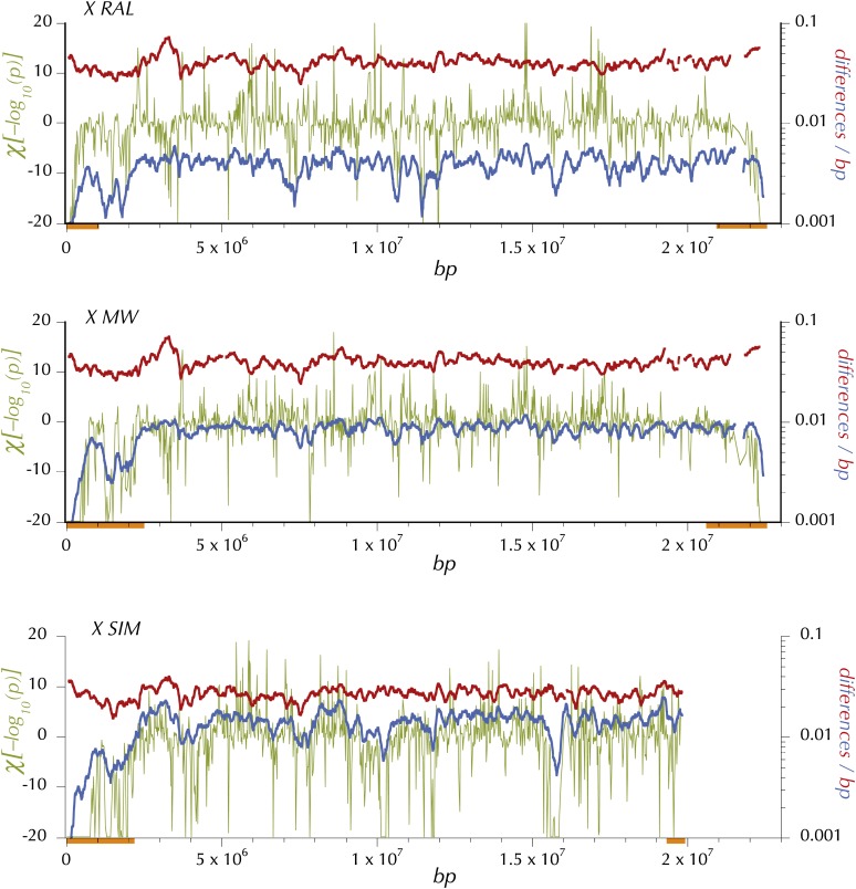
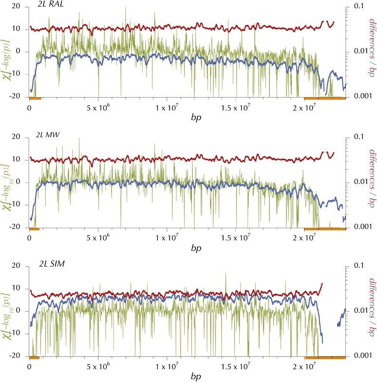
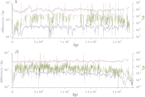
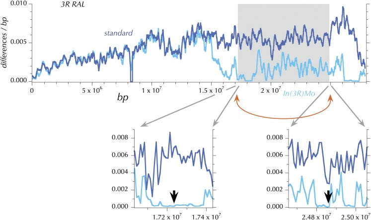
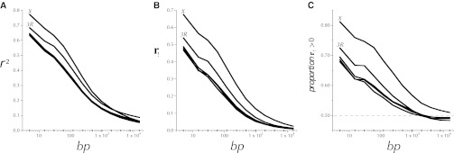
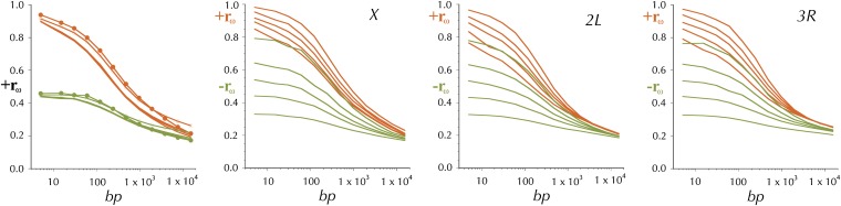
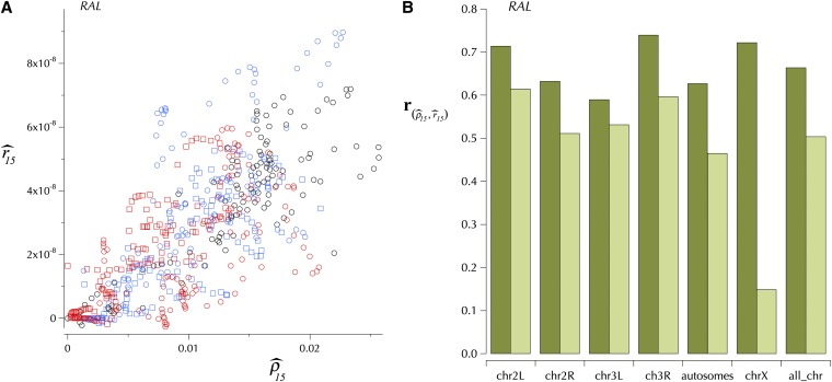
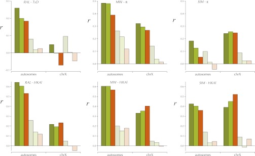
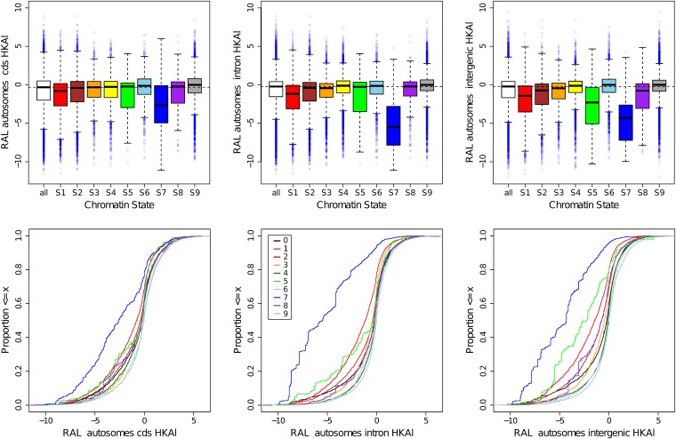
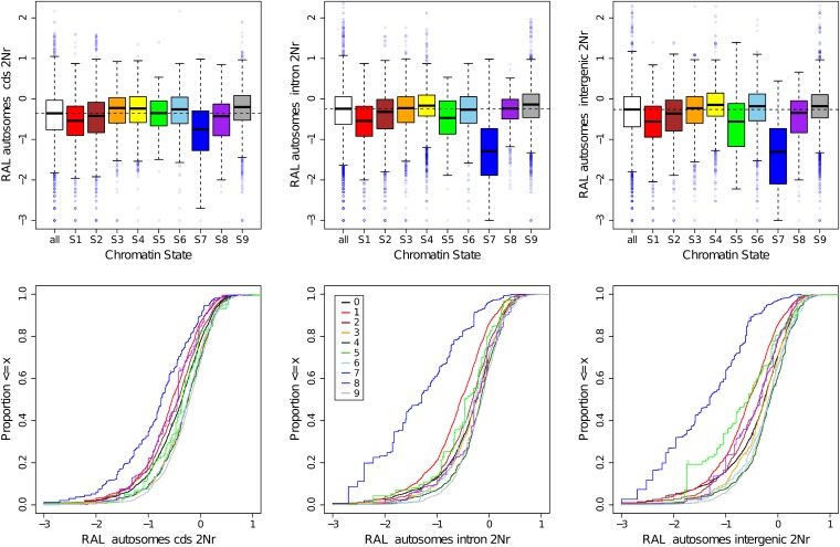
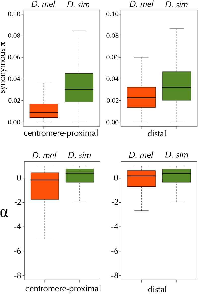
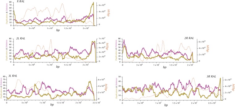
This report of independent genome sequences of two natural populations of Drosophila melanogaster (37 from North America and 6 from Africa) provides unique insight into forces shaping genomic polymorphism and divergence. Evidence of interactions between natural selection and genetic linkage is abundant not only in centromere- and telomere-proximal regions, but also throughout the euchromatic arms. Linkage disequilibrium, which decays within 1 kbp, exhibits a strong bias toward coupling of the more frequent alleles and provides a high-resolution map of recombination rate. The juxtaposition of population genetics statistics in small genomic windows with gene structures and chromatin states yields a rich, high-resolution annotation, including the following: (1) 5'- and 3'-UTRs are enriched for regions of reduced polymorphism relative to lineage-specific divergence; (2) exons overlap with windows of excess relative polymorphism; (3) epigenetic marks associated with active transcription initiation sites overlap with regions of reduced relative polymorphism and relatively reduced estimates of the rate of recombination; (4) the rate of adaptive nonsynonymous fixation increases with the rate of crossing over per base pair; and (5) both duplications and deletions are enriched near origins of replication and their density correlates negatively with the rate of crossing over. Available demographic models of X and autosome descent cannot account for the increased divergence on the X and loss of diversity associated with the out-of-Africa migration. Comparison of the variation among these genomes to variation among genomes from D. simulans suggests that many targets of directional selection are shared between these species.

Figure 1

SNP rate (differences from the reference sequence per base pair) of the RAL lines for base pairs with different Illumina quality scores, ≥Q10, ≥Q20, ≥Q30, and ≥Q40 (light to dark blue) plotted with depth-weighted mean GC content at unique base pairs (large solid circles). The whiskers show the range of depth-weighted GC content over lanes. The gray bars show depth-weighted %GC of the median lane. Note the apparent increase in nonreference basecalls (SNP rate) in the lines with the lowest GC content.

Figure 2

The distributions of observed and simulated HKAl (signed chi-square) values. The olive line is the distribution of observed HKAl values for all adjacent windows of 50 variant sites (segregating or fixations on the melanogaster lineage) for which the expected numbers derive from the observed averages in the large subset of these windows outside the designated (“trimmed”) centromere- and telomere-proximal regions with low crossing over. The black line shows the distribution of HKAl for the same windows, using the observed averages for all windows to derive the expected numbers. The blue and red lines are the theoretical distributions for high and no recombination derived from simulations using Hudson’s ms program with the commands ms 35 1000000 -s 50 -r 8 500 -I 2 1 34 -ej 2.5 1 2 or -r 0, respectively. The parameter -ej 2.5 relates the outgroup divergence time to 4N₀ and yields the observed proportion of segregating sites (0.44), both averaged over all sample sizes and only at sites with 34 observed alleles, the simulated number.

Figure 3

Distributions of estimates of the rates of recombination per base pair, r (M/bp) and ρ = 2Nr, where N is the populations size (see text). ${\widehat{r}}_{15}$ is the (orange) loess-smoothed (span = 15%) per genome per generation estimate of the rate of recombination between adjacent base pairs, derived from curated FlyBase genetic map positions. (A) ${\widehat{r}}_{15}$ and the estimated r for each subdivision on the X, plotted on a logarithmic scale. ${\widehat{\rho }}_{15}$ is the (olive) comparably (span = 15%) loess-smoothed per population per generation estimate of the rate of recombination (2Nr) between adjacent base pairs (see text). The gray line is the higher-resolution (span = 8%) smoothed estimate of 2Nr, ${\widehat{\rho }}_8$.

Figure 4

The distributions of estimates of expected heterozygosity and of divergence in 1000-bp windows on chromosome arms (X, 2L, 2R, 3L, and 3R) for RAL, MW, and SIM.

Figure 5

Expected heterozygosity, divergence, and HKAl on the X for the North American (RAL), African (MW), and simulans (SIM) samples. Blue shows expected heterozygosity, π at the midpoint of 150-kbp windows (incremented every 10 kbp, minimum coverage = 0.25 and Q30 sequence). Red shows lineage-specific, average Q30 divergence in 150-kbp windows (incremented every 10 kbp and minimum coverage of 0.25). A preliminary application of HKAl on the Q30 data in windows of 4096 contiguous polymorphic or divergent sites identified centromere- and telomere-proximal regions (orange bars) in which the each window exhibited a deficiency of polymorphic sites relative to the chromosome-arm average. Then HKAl was applied again on the Q30 data in windows of 512 contiguous polymorphic or divergent sites (excluding these centromere- and telomere-proximal regions from calculation of the chromosome-arm–wide expected proportions, p_c and d_c). χ[log(p_HKAl)] (olive) is the log of the P-value associated with HKAl plotted with the sign of the difference between the observed number and the expected number of polymorphic sites in the window.

Figure 6

Expected heterozygosity, π_w, divergence, δ_w, and HKAl on 2L for the North American (RAL), African (MW), and simulans (SIM) samples. Blue shows expected heterozygosity, π_w at the midpoint of 150-kbp windows (incremented every 10 kbp, minimum coverage = 0.25 and Q30 sequence). Red shows lineage-specific, Q30 divergence, δ_w in 150-kbp windows (incremented every 10 kbp and minimum coverage of 0.25). A preliminary application of HKAl on the Q30 data in windows of 4096 contiguous polymorphic or divergent sites identified centromere- and telomere-proximal regions (orange bars) in which the each window exhibited a deficiency of polymorphic sites relative to the chromosome-arm average. Then HKAl was applied to the Q30 data in windows of 512 contiguous polymorphic or divergent sites (excluding these centromere-and telomere-proximal regions from calculation of the chromosome-arm–wide expected proportions, p_c and d_c). χ[log(p_HKAl)] (olive) is the logarythim of the P-value associated with the HKAl plotted with the sign of the difference between the observed number and the expected number of polymorphic sited in nonoverlapping windows of 512 variable sites.

Figure 7

$\widehat{\rho }$, estimates of 2Nr across chromosome arms X and 2L, generated by LDhat. Also shown for comparison are estimates of π_w (blue) and δ_w (red) as in Figures 5 and 6 (see Figure S7 for this type of plot for all five chromosome arms).

Figure 8

Expected heterozygosity, π_w on 3R for the North American (RAL) sample. The dark blue line shows expected heterozygosity, π_w at the midpoint of 150-kbp windows (incremented every 10 kbp and Q30 sequence) for the “standard” arrangements in the RAL sample. The light blue line is the comparable plot for the In(3R)Mo arrangements of chromosome 3R in the RAL sample. The gray rectangle demarcates the inverted region in In(3R)Mo. The two insets below are blow-ups of the genomic regions surrounding the two breakpoints marked by arrows (Corbett-Detig et al. 2012).

Figure 9

(A–C) The decay of linkage disequilibrium with physical distance on the chromosome arms in the North American sample (RAL) of D. melanogaster. The average r² between all pairs of Q30 SNPs with minor allele frequency (MAF) ≥0.167 separated by contiguous ranges of base pairs is plotted in A against the midpoint of each range (indicated by the dots on the abscissa). The ranges are [1, 10] and (s_i−1, s_i], for 1 < i ≤ 12, where s_i = 10, 20, 40, 80, 160, 320, 640, 1280, 2560, 5120, 10,240, and 20,480. The lines for the X and 3R are distinct from those for 2L, 2R, and 3L and are labeled. B shows the distribution of the average allele-frequency–oriented correlation coeffficent, r_ω over the same intervals for each chromosome arm (see Table 1 for the definition of r_ω). And C shows that much of the shift toward more positive r_ω is attributable to an increase in the proportion of pairs of SNPs with r_ω > 0.

Figure 10

The distribution of positive and negative average r_ω at different distances (bp) for pairs of Q30 SNPs in the North American (RAL) sample. The left plot shows the pattern for the five large chromosome arms, orange is the average r_ω > 0, and olive is the average r_ω < 0, where the MAF ≥ 0.167. Solid circles mark the X, while open circles are 3R. The other three chromosome arms are hardly distinguishable. The right three panels are plots similar to the first (left) but for chromosome arms X, 3R, and 2L. The different lines of r_ω > 0 (orange) and r_ω < 0 (olive) correspond to subsets in which p(1 − p)q(1 − q), the product of the SNP allele frequencies at each locus (p and q) fall in the following intervals, respectively (increasing in r_ω): 0.0255–0.0383, 0.0383–0.0468, 0.0468–0.0531, 0.0531–0.0582, and 0.0582–0.0625.

Figure 11

Common patterns of the genomic distribution of the two estimates of the rate of recombination per base pair, ${\widehat{r}}_{15}$ and ${\widehat{\rho }}_{15}$. (A) A scatterplot of these two estimates in windows of variable sizes (all >10⁴ bp) for each of the untrimmed chromosome arms. Eight outliers are off this plot (2R, −0.0027, −6.2 × 10⁻⁹; X, 0.0321, 1.9 × 10⁻⁸; 0.0375, 2.2 × 10⁻⁸; 0.0400, 2.5 × 10⁻⁸; 0.0404, 2.7 × 10⁻⁸; 0.0373, 3.0 × 10⁻⁸; 0.0314, 3.3 × 10⁻⁸; 0.0275, 3.7 × 10⁻⁸). B compares the base pair-weighted correlation logarithms of ${\widehat{r}}_{15}$ and ${\widehat{\rho }}_{15}$, ${\mathit{r}}_{\widehat{\rho }\mathrm{,}\widehat{r}}$ among chromosome arms for both trimmed (light green) and untrimmed (dark green). The parallels between the two measures are high, but reduced slightly when only the trimmed regions are considered. This is not true for chromosome X, which shows much less correlation between the two estimates on the trimmed data.

Figure 12

Correlations between recombination rates and HKAl, π_w, and TsD. r is the base pair-weighted Pearson’s correlation coefficient between TsD, π_w, and HKAl and the logarithm of ${\widehat{\rho }}_0$ (olive), ${\widehat{\rho }}_{15}$ (light olive), and ${\widehat{r}}_{15}$ (orange) across the autosomes and the X chromosome. The three lower columns to the right (lighter shades) are the corresponding correlations for the “trimmed” euchromatic regions (see text and Table S15 and Figure S8).

Figure 13

The distribution of (“untrimmed”) HKAl values in windows partitioned by chromatin state (inferred from S2 cells) and gene structure (coding, intron, and intergenic). The top row shows box plots (boxes are the central two quartiles, the whiskers are 1.5 times those, and the dots with light shading represent the outliers beyond the whiskers). The empirical cumulative distribution functions (ecdfs) in the bottom row give a perhaps clearer alternative view of the differences in the distributions of HKAl between chromatin states in the coding, intronic, and intergenic regions. Also see Figure S11 and Figure S12 for the box plots and ecdfs (respectively) for π_w (RAL, MW, and SIM), δ_w (RAL, MW, and SIM), HKAl (RAL, MW, and SIM), HBKl, and $\widehat{\rho }$. “all” in the box plots and “0” in the ecdfs refer to the sum of the chromatin states, 1–9.

Figure 14

The distribution of $\widehat{\rho }$-values in windows partitioned by chromatin state inferred in S2 cells and gene structure (coding, intron, and intergenic). The top row shows box plots (boxes are the central two quartiles, the whiskers are 1.5 times those, and the dots with light shading represent the outliers beyond the whiskers). The empirical cumulative distribution functions (ecdfs) in the bottom row give a perhaps clearer alternative view of the differences in the distributions of $\widehat{\rho }$ between chromatin states in the coding, intronic, and intergenic regions. Also see Figure S11 and Figure S12 for the box plots and ecdfs (respectively) for π_w (RAL, MW, and SIM), δ_w (RAL, MW, and SIM), HKAl (RAL, MW, and SIM), HBKl, and $\widehat{\rho }$. “all” in the box plots and “0” in the ecdfs refer to the sum of the chromatin states, 1–9.

Figure 15

Comparisons of the levels of synonymous polymorphism (π_s) and the proportions of amino acid fixations driven by positive selection (α) in centromere-proximal and distal regions of the autosomes of D. melanogaster (shown in olive) and D. simulans (shown in orange). Using the ${\widehat{r}}_{15}$-smoothed map of the recombination rate, the boundaries between the centromere-proximal and distal regions were chosen to be the first interval where ${\widehat{r}}_{15}$ > 1.8 × 10⁻⁸ M/bp, 4,714,046 for 2L, 9,716,832 for 2R, 2,350,586 for 3L, and 13,015,705 for 3R.

Figure 16

The distribution of duplications and deletions in 1-Mbp windows spaced every 100 kbp across the X and autosomes. To smooth the underlying count data from independent nonoverlapping 100-kbp windows, windows >3 standard deviations from the mean and with <40% consensus sequence coverage were filtered. These nonoverlapping windows were then averaged using a 1-Mb sliding window spaced every 100 kbp. The genomic distribution of ${\widehat{r}}_{15}$ is added for comparison.

Figure 17

The proportion of duplications (solid bars) and deletions (open bars) containing at least one entire gene, containing a portion of an exon (coding or noncoding), containing an intronic segment, or containing only intergenic regions. Note that deletions are far less likely than duplications to contain whole genes or exonic segments. Instead, deletions are disproportionately found within intergenic regions. Duplications, on the other hand, do not appear to be biased toward intergenic regions (which make up ∼35% of the genome).

Figure 18

The distribution of HKAl outliers along gene regions and among functional classes of sites. The number of outlier windows centering on each gene position bin (A and C) or functional element (B and D) was compared against the total number of analyzed windows centering on each of these categories for MW HKAl, for low outliers (A and B) and high outliers (C and D). Over- and underrepresentation of each category was calculated such that a value of 1 matches the random genome-wide expectation, while a value of 2 indicates twice as many HKAl outliers in this category as expected randomly. Gene positions (A and C) were defined with regard to the beginning of the 5′-UTR and the end of the 3′-UTR. “kbp” bins indicate distance upstream or downstream of these limits, while genic bins indicate relative position between these limits and encompass 5′-UTR, coding exon, intron, and 3′-UTR sequences. These categories are depicted separately, along with proximal intergenic (within 2 kbp of a gene) and distal intergenic regions, in B and D.

Figure A1

Interior score MaxIS. An interior score is defined for each position in a read (open boxes) as the distance to the nearest edge. It follows that each nucleotide in the consensus sequence has a corresponding set of interior scores that overlap it. To compute MaxIS, the consensus sequence (shaded boxes) inherits the maximum max() of the interior scores of the overlapping reads. SumIS and AveIS are defined by replacing the max() function with sum() and ave(), respectively.

Figure A2

ROCs for the simple models (see text). Cumulative coverage (y-axis) vs. observed error rate (x-axis) is plotted for the model based only on Q (red) and the seven extensions based on the addition of a single (indicated) predictor variable. Note the improvement of the discrimination achieved with several of the extensions.

Figure A3

Quantile error rates for predictor variables: right, $\widehat{Q}$ vs. depth; center, $\widehat{Q}$ vs. MinQ5; and left, $\widehat{Q}$ vs. MaxIS. The mean empirical quality score $\widehat{Q}$ (y-axis) was calculated in quantiles large enough to estimate $\widehat{Q}$ (see text). The quantile mean of predictor variables is plotted on the x-axis.

Figure A4

ROC for selected model (cumulative coverage vs. cumulative error rate, parameterized by the quality score cutoff). The final quality score model and three earlier models incorporating the individual components are compared to the initial MAQ quality scores Q.

Figure A5

Empirical quality (y-axis) vs. the consensus quality score Q (x-axis) from the MAQ assemblies of both ycnbwsp assemblies (one purple and one orange). The ideal relationship between the idealized quality score and the empirical quality is shown with the red line. The final recalibrated consensus quality scores for both ycnbwsp assemblies are plotted in green and blue. The recalibrated consensus quality scores show improved accuracy as they are much closer to the ideal relationship. See text.

Figure B1

P_L(γ) vs γ (see Equation B1). The solid line represents the mean of the G+C profiles of all stocks in the CNV analysis. The dashed lines are ±1 standard deviation.

Figure B2

P_L(γ) vs γ (see Equation B1). The lines represent the library specific G+C profiles of all stocks in the CNV analysis.

Figure B3

X/A ratios. Here we plot $E\left(\text{read}\hspace{0.17em}\text{depth}\hspace{0.17em}\text{in}\hspace{0.17em}\text{window}\right|\text{window}\hspace{0.17em}\text{is}\hspace{0.17em}\text{on}\hspace{0.17em}\text{X})/ E\left(\text{read}\hspace{0.17em}\text{depth}\hspace{0.17em}\text{in}\hspace{0.17em}\text{window}\right|\text{window}\hspace{0.17em}\text{is}\hspace{0.17em}\text{on}\hspace{0.17em}\text{A})$ estimated for all stocks. Values fall in the expected range between 1 (all females) and 3/4 (50% males).

Figure B4

Shown here are the aberrant library compositional profiles P_L(γ) vs γ (see Equation B1) for RAL-379, RAL-313, and MW9-1. These were removed from subsequent analysis of copy-number variation.

Figure B5

Variance in windowed read depth (y-axis) vs the predicted mean read depth (x-axis) for RAL-689 using Equation B3. Overdispersion was quantified by estimating a dispersion parameter η where σ² = ηλ. The dispersion parameter η was estimated by regression through the origin. In the case of RAL-689, η = 2.03.

Figure B6

Dispersion parameter (η) estimates for all stocks. The stocks removed due to aberrant G+C profiles are labeled and cluster above η = 4. Using that information as an empirical guideline, all stocks with η > 4 were removed from subsequent analyses on the basis of overdispersion.

Figure B7

Scatterplot showing the association of the variance with the mean of read depth.

References

1. Adams M. D., Celniker S. E., Holt C. A., Evans J. D., Gocayne J. D., et al. , 2000. The genome sequence of Drosophila melanogaster. Science 287: 2185–2195 - PubMed
1. Aguadé M., Miyashita N., Langley C. H., 1989. Reduced variation in the yellow-achaete-scute region in natural populations of Drosophila melanogaster. Genetics 122: 607–615 - PMC - PubMed
1. Aguadé M., Meyers W., Long A. D., Langley C. H., 1994. Single-strand conformation polymorphism analysis coupled with stratified DNA sequencing reveals reduced sequence variation in the su(s) and su(wa) regions of the Drosophila melanogaster X chromosome. Proc. Natl. Acad. Sci. USA 91: 4658–4662 - PMC - PubMed
1. Akashi H., 1995. Inferring weak selection from patterns of polymorphism and divergence at “silent” sites in Drosophila DNA. Genetics 139: 1067–1076 - PMC - PubMed
1. Akashi H., 1996. Molecular evolution between Drosophila melanogaster and D. simulans: reduced codon bias, faster rates of amino acid substitution, and larger proteins in D. melanogaster. Genetics 144: 1297–1307 - PMC - PubMed
Publication types
LinkOut - more resources