Parallel MR imaging

Abstract

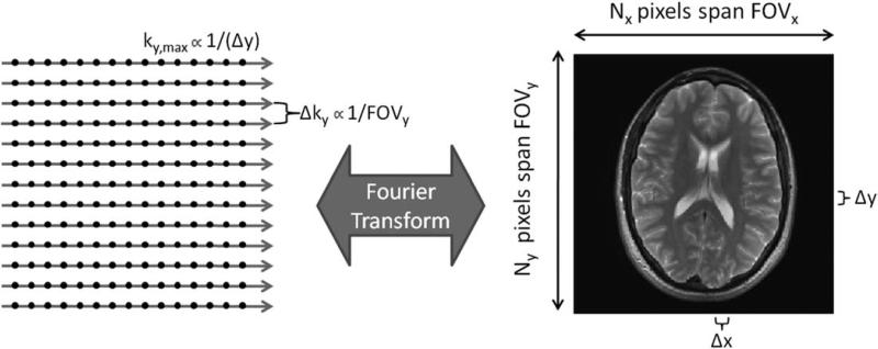
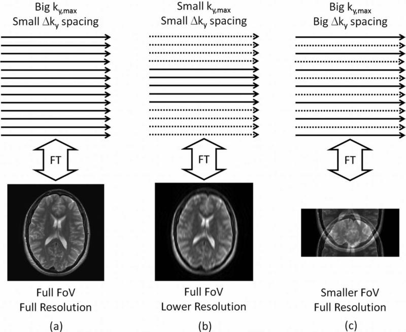
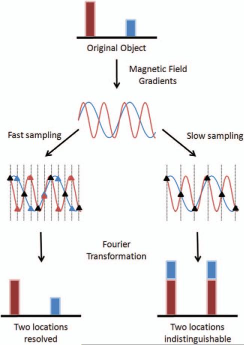
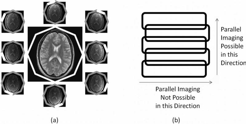
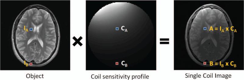
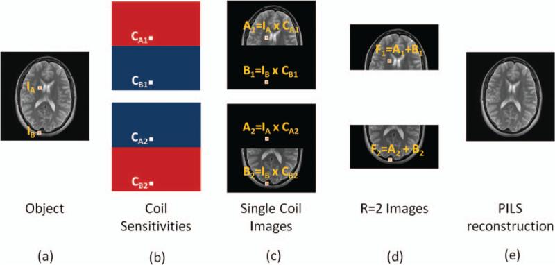
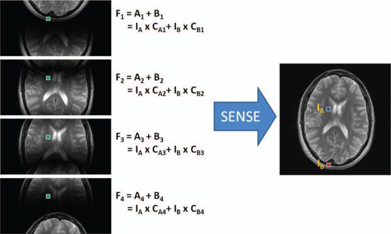
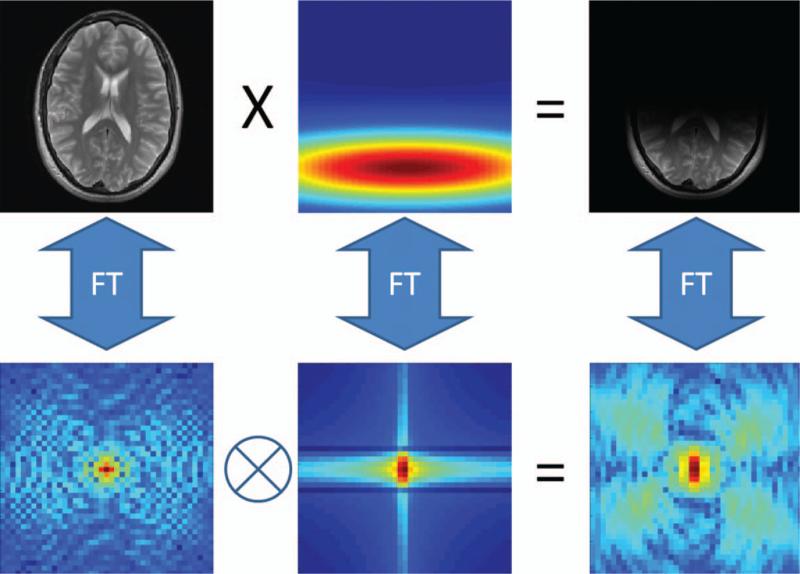
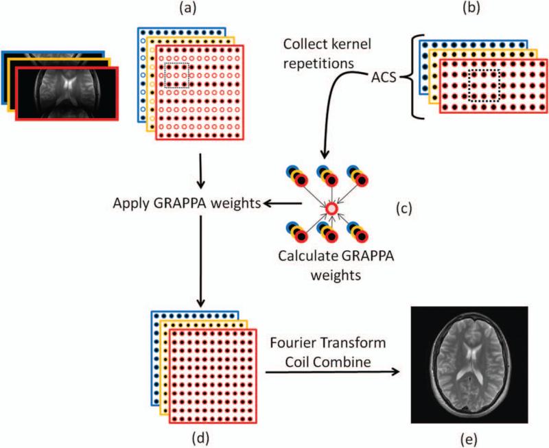
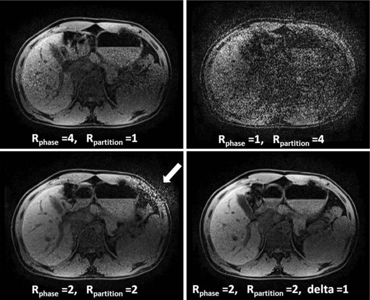
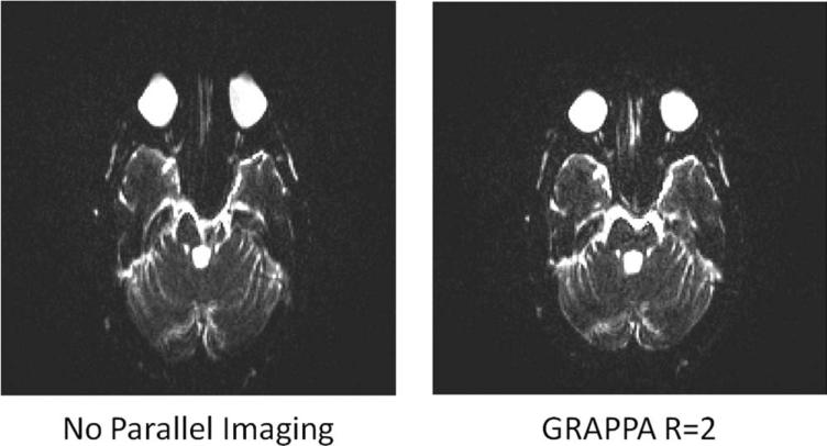
Parallel imaging is a robust method for accelerating the acquisition of magnetic resonance imaging (MRI) data, and has made possible many new applications of MR imaging. Parallel imaging works by acquiring a reduced amount of k-space data with an array of receiver coils. These undersampled data can be acquired more quickly, but the undersampling leads to aliased images. One of several parallel imaging algorithms can then be used to reconstruct artifact-free images from either the aliased images (SENSE-type reconstruction) or from the undersampled data (GRAPPA-type reconstruction). The advantages of parallel imaging in a clinical setting include faster image acquisition, which can be used, for instance, to shorten breath-hold times resulting in fewer motion-corrupted examinations. In this article the basic concepts behind parallel imaging are introduced. The relationship between undersampling and aliasing is discussed and two commonly used parallel imaging methods, SENSE and GRAPPA, are explained in detail. Examples of artifacts arising from parallel imaging are shown and ways to detect and mitigate these artifacts are described. Finally, several current applications of parallel imaging are presented and recent advancements and promising research in parallel imaging are briefly reviewed.

Figure 1

Data in k-space are usually collected on a Cartesian grid (left). The Fourier transform is used to convert the k-space to an image of size N_x by N_y pixels (right). The extent of k-space covered (k_x,max and k_y,max) is inversely proportional to the image resolution (Δx and Δy). The spacing between adjacent samples in k-space (Δk_x and Δk_y) is inversely proportional to the field-of-view (FOV_x and FOV_y).

Figure 2

a: A high-resolution image covering the full FOV requires collection of data along closely-spaced lines that span a large region of k-space. b: Reducing k_y,max maintains the FOV but decreases the image resolution. c: Increasing Δk_y while holding k_y,max constant maintains image resolution but decreases the FOV, resulting in spatial aliasing artifacts in the corresponding image.

Figure 3

A 1D object with two signal sources at two different locations (red and blue in the top row) gives rise to two signals oscillating at different frequencies (second row). These signals are sampled at a high rate (third row left) and at a lower rate (third row right), where the sampling time is indicated by vertical dotted lines. The points sampled are denoted as triangles; at some sampling times, the two signals appear the same (black triangles). If the signals are sampled at a high enough rate (left bottom), the frequencies can be distinguished from one another and the two locations can be resolved. If the signals are sampled too slowly (right bottom), or undersampled, the two frequencies appear the same at these sampled points and the two locations cannot be distinguished.

Figure 4

(a) An example head coil array made up of eight independent receiver coils arranged around the object in a circle. Each coil is more sensitive to signal originating from the tissue closest to it, and can be used to form its own image (small images). The independent coil images can be combined into a single image with uniform sensitivity (large center image). (b) An example linear array made up of five coils, where the sensitivity profile of each array is similar in the horizontal direction, but the sensitivity decreases with distance along the vertical direction. When using such a coil, acceleration can only be performed in the vertical direction where there is substantial variation in the coil sensitivities.

Figure 5

The object pixels (left) are weighted, ie, multiplied, by the sensitivity of the receiver coil (center) to yield the single-coil image (right).

Figure 6

The data acquisition for the object shown in (a) can be performed using a two-channel receiver array (b) where each receiver is sensitive to a localized region and sensitivity regions do not overlap. Each receiver coil gives rise to one fully sampled image where each pixel is the product of the object location and the coil sensitivity map (c). In the case of B₁, for instance, the coil sensitivity value at location B, namely C_B1, is zero. If the scan is accelerated by a factor of 2, the FOV in each single-coil image is decreased by a factor of 2 (d). These accelerated single-coil images are aliased (pixel F₁ is the sum of pixels A₁ and B₁), but because one of the aliased pixels comes from outside the region of sensitivity, it will contribute no overlapping signal. The full FOV image can be reconstructed by piecing together the accelerated single-coil images (e).

Figure 7

A four-channel linear array is used to acquire an image with acceleration factor R = 2. This results in four single-coil images where two pixels, I_A and I_B, are aliased. The aliased pixels, F₁ through F₄, in each single-coil image are sums of the two pixels weighted by the appropriate coil sensitivity values. Given that the coil sensitivity values (the C_A and C_B terms) are known, SENSE solves the resulting system of equations with four known values (F₁, F₂, F₃, and F₄) and two unknown values (I_A and I_B) to unfold the aliased single-coil images into a full FOV image. [Color figure can be viewed in the online issue, which is available at wileyonlinelibrary.com.]

Figure 8

In the image domain (top row), a fully sampled image (left) multiplied by a localized coil sensitivity profile (center) results in a single-coil image (right). Looking at the same relationship in k-space (bottom row), the k-space of the object (left) is smeared (or convolved) with the k-space of the coil sensitivity (center), resulting in spreading of the k-space data across several points in the single-coil k-space (right).

Figure 9

a: Undersampled k-space data are collected from each coil, where the different coils are shown with different colors. The kernel (outlined by the dotted black box) consisting of some source points (solid circles) and target points (empty circles) defines the neighborhood of k-space points that will be used for the GRAPPA reconstruction. b: Additional data (auto-calibration signals, or ACS) are collected, usually near the center of k-space. c: The repetitions of the kernel through the ACS region are used to calculate the GRAPPA weights. d: The GRAPPA weights are then applied to fill in the missing k-space data from each coil to produce fully sampled single-coil data. e: The Fourier transform is used to obtain single-coil images, which are then combined to form a reconstructed full-FOV image. [Color figure can be viewed in the online issue, which is available at wileyonlinelibrary.com.]

Figure 10

Examples of R = 4 GRAPPA kernel patterns for 3D imaging, where the black points are the source points and the gray points are the target points. The phase-encoding direction is up-down, the partition-encoding direction is left-right, and the frequency-encoding (or read) direction is into the plane of the page. a: The entire R = 4 acceleration is performed in the phase-encoding direction, which can lead to residual aliasing artifacts and high g-factor losses depending on the coil configuration. b: The acceleration has been split up such that the phase and partition-encoding directions each experience R = 2, leading to a total acceleration of R = 4. This type of acceleration can lead to an improved image quality compared to the pattern in (a). c: A CAIPIRINHA pattern, where the acceleration has been split up as in (b), but the acquired points are offset (the so-called R_phase = 2, R_partition = 2, delta = 1 pattern). Such a pattern causes the aliasing to be shifted and can lead to lower g-factors and more robust GRAPPA reconstructions than the patterns in either (a) or (b).

Figure 11

Example GRAPPA reconstructions of head images using acceleration factors R = 2, R = 3, and R = 4 and 24 ACS lines. A total of 12 receiver coils were used to acquire these data. Note that as the acceleration factor increases, the noise enhancement increases (compare R = 2 and R = 3), and residual aliasing artifacts start to appear (R = 4). Similar artifacts appear in the equivalent SENSE reconstructions.

Figure 12

T₁-weighted abdominal images acquired with R = 3 (left) and R = 2 (right) in the up-down direction and reconstructed using GRAPPA. Note the residual aliasing in the left image, which could appear to be abnormal vasculature in the liver lesion. Decreasing the acceleration factor removes these artifacts, as can be seen in the image on the right.

Figure 13

Examples of GRAPPA-reconstructed partitions from a 3D abdominal scan with acceleration factors of R = 4. Top left: All of the acceleration is performed in the phase-encoding direction (up-down), leading to noise enhancement (GRAPPA kernel shown in Fig. 10a). Top right: All of the acceleration is performed in the partition-encoding direction (head-foot). Because the coil array is more suited to acceleration in the up-down direction, this arrangement leads to a poorer reconstruction than when accelerating only in the phase-encoding direction. Bottom left: The acceleration has been split up between the phase and partition-encoding directions (kernel shown in Fig. 10b), thereby improving the reconstruction quality. Note the residual aliasing artifacts outside the body near the stomach and spleen. Bottom right: By using a CAIPIRINHA pattern where the acquired k-space points are offset with respect to one another (kernel shown in Fig. 10c), the g-factor is reduced and a clinically acceptable R = 4 image is generated.

Figure 14

Left: The long echo train length of an unaccelerated EPI sequence used in diffusion-weighted imaging creates severe geometric distortions. Right: The use of parallel imaging allows for a shortened echo train length, thereby reducing geometric distortions and restoring the image to diagnostic quality.

References

1. Pruessmann KP, Weiger M, Scheidegger MB, Boesiger P. SENSE: sensitivity encoding for fast MRI. Magn Reson Med. 1999;42:952–962. - PubMed
1. Griswold MA, Jakob PM, Heidemann RM, et al. Generalized autocalibrating partially parallel acquisitions (GRAPPA). Magn Reson Med. 2002;47:1202–1210. - PubMed
1. Paschal CB, Morris CB. K-space in the clinic. J Magn Reson Imaging. 2004;19:145–159. - PubMed
1. Cohen MS, Weisskoff RM, Rzedzian RR, Kantor HL. Sensory stimulation by time-varying magnetic fields. Magn Reson Med. 1990;14:409–414. - PubMed
1. Ham CL, Engels JM, van de Wiel GT, Machielsen A. Peripheral nerve stimulation during MRI: effects of high gradient amplitudes and switching rates. J Magn Reson Imaging. 1997;7:933–937. - PubMed