Live imaging using adaptive optics with fluorescent protein guide-stars

Abstract

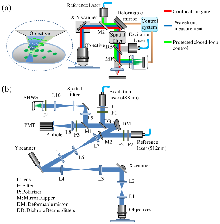
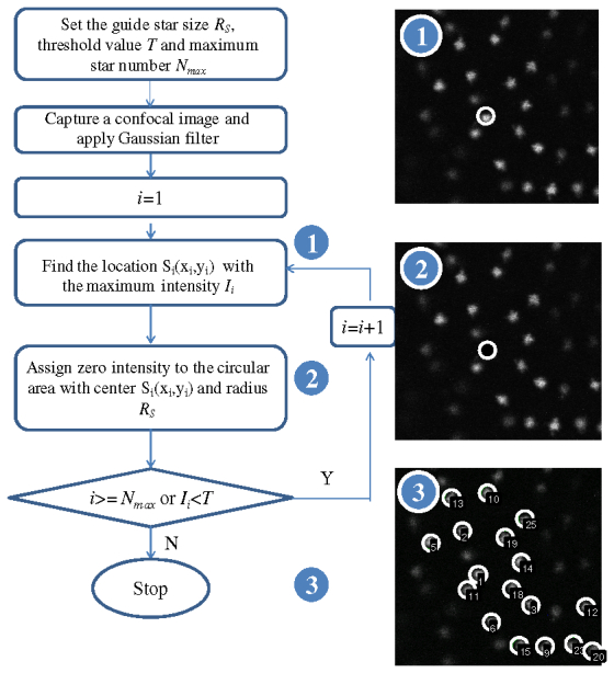
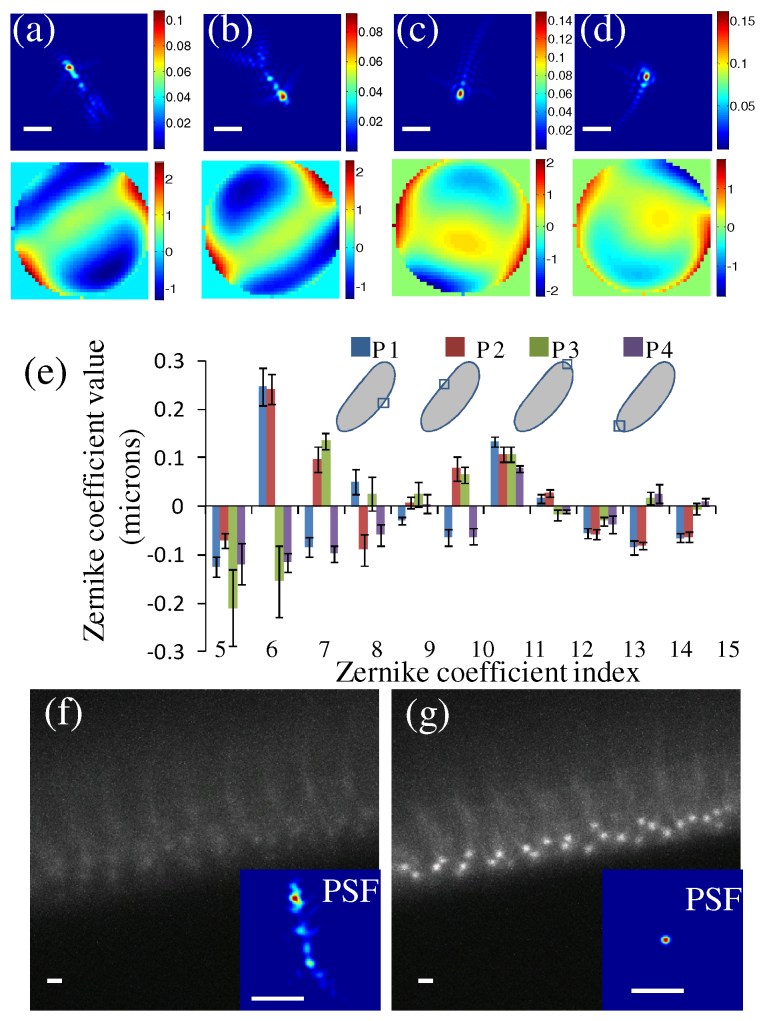
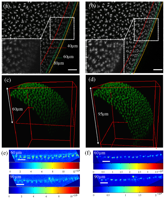
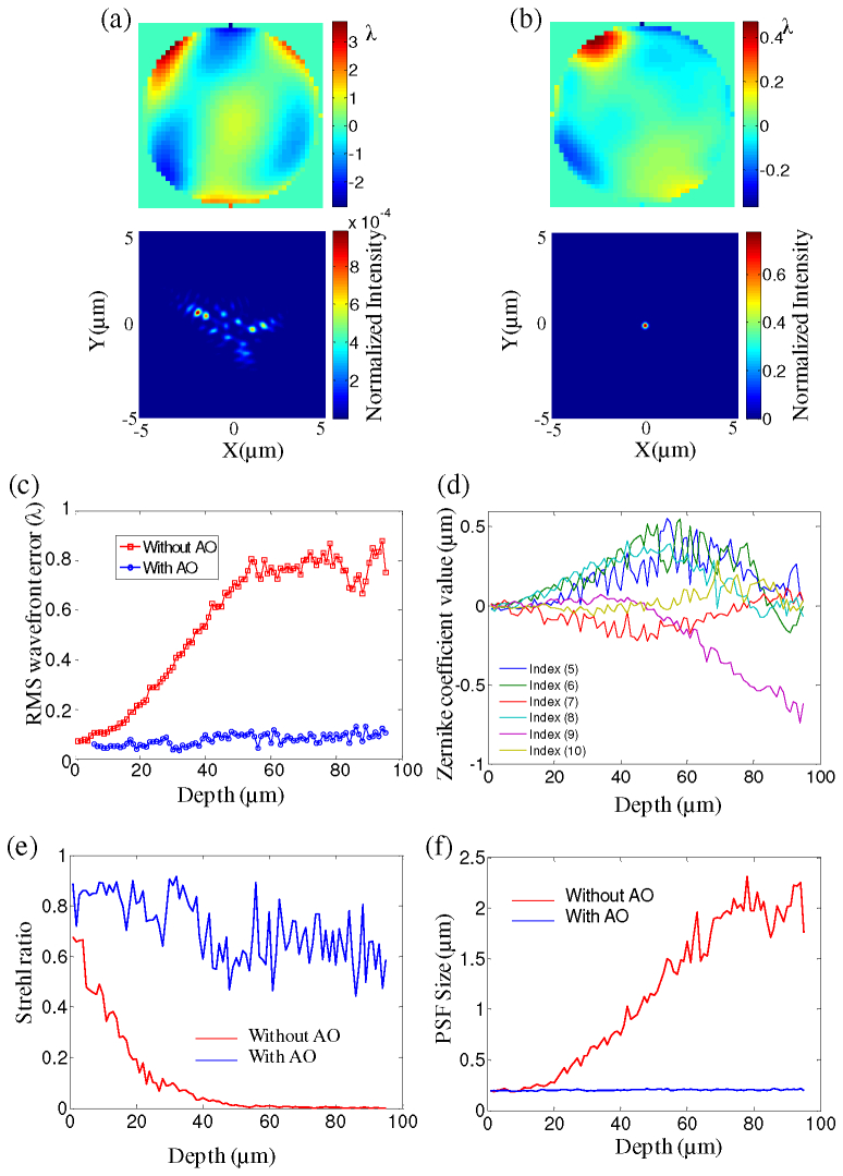
Spatially and temporally dependent optical aberrations induced by the inhomogeneous refractive index of live samples limit the resolution of live dynamic imaging. We introduce an adaptive optical microscope with a direct wavefront sensing method using a Shack-Hartmann wavefront sensor and fluorescent protein guide-stars for live imaging. The results of imaging Drosophila embryos demonstrate its ability to correct aberrations and achieve near diffraction limited images of medial sections of large Drosophila embryos. GFP-polo labeled centrosomes can be observed clearly after correction but cannot be observed before correction. Four dimensional time lapse images are achieved with the correction of dynamic aberrations. These studies also demonstrate that the GFP-tagged centrosome proteins, Polo and Cnn, serve as excellent biological guide-stars for adaptive optics based microscopy.

Fig. 1

System setup. (a) Schematic diagram of the AOM: GFPs are illuminated with an excitation laser (488 nm) to produce a guide-star. The reference laser is used for wavefront control. The flip mirrors M1 and M2 control the light path for confocal imaging (red), wavefront measurement (blue) and protected closed-loop control of the DM (green). (b) Experimental set-up of the AOM. L, lens; F, filter; P, polarizer; M, mirror flipper; DM, deformable mirror; DB, dichroic beamplitters.

Fig. 2

Flowchart for the guide-star searching algorithm. The algorithm is to search and calculate the locations of the possible guide-stars stars in the image.

Fig. 3

Measurement noise change with the exposure time at different depths. The error bar is the standard deviation for 10 measurements.

Fig. 4

Wavefront measurement and correction. (a-d) The averaged point spread function (PSF) and wavefront errors over 6 measurements using EGFP-Cnn labeled centrosomes of a cycle 14 Drosophila embryo at four different locations (P1, P2, P3 and P4) at a depth of 60 µm. (e) The averaged coefficient value of the first 15 Zernike polynomial modes at these four locations. The error bar is the standard deviation for 6 measurements. (f-g) The images and PSF without and with correction for a cycle 14 Drosophila embryo with GFP-polo at a depth of 83 μm. Scale bars, 2 µm.

Fig. 5

Comparison of the three-dimensional imaging without and with correction for imaging of cycle 13 fly embryos with EGFP-Cnn label. (a-b) The maximum intensity projection of the scan series from the top surface to 100 μm without and with AO ( Media 1). (c-d) The 3D reconstructions without and with AO. (e-f) The confocal images without and with AO at the depths of 60 μm and 90 μm. The color maps are scaled to show the image data over its full range. Scale bar, 10 µm.

Fig. 6

Comparison of the wavefront measurements and the PSFs without and with AO for different depths. (a-b) The wavefront measurements and PSF without and with AO at the depth of 90 μm ( Media 2). (c) The RMS wavefront errors change with the depth. The red and blue lines indicate the measurement without and with AO respectively. (d) The Zernike coefficient values without AO with the change of depth. (e-f) The Strehl ratio and PSF size change for different depths. The red and blue lines indicate without and with AO respectively. (λ = 509 nm)

Fig. 7

4D imaging of cycle 13 fly embryos with EGFP-Cnn label at depth of 80 µm. (a) A single frame without and with correction of a video movie ( Media 3). (b) The coefficient value changes for Zernike modes $z_2^2$ (Astigmatism x, dashed line) and $z_3^{-3}$ (Trefoil y, solid line) with and without AO during 20 minutes. (c) The Strehl ratio change with (blue) and without (red) AO during 20 minutes. (d) PSF size change with (blue) and without (red) AO during 20 minutes ( Media 4).

References

1. Booth M. J., “Adaptive optics in microscopy,” Phil. Trans. R. Soc. A–Math. Phys. Eng. Sci. 365, 2829–2843 (2007). - PubMed
1. R. K. Tyson, Principles of Adaptive Optics (Academic, 1991).
1. J. Porter, H. Queener, J. Lin, K. Thorn, and A. A. S. Awwal, Adaptive Optics for Vision Science: Principles, Practices, Design and Applications, (Wiley, 2006).
1. Marsh P., Burns D., Girkin J., “Practical implementation of adaptive optics in multiphoton microscopy,” Opt. Express 11(10), 1123–1130 (2003).10.1364/OE.11.001123 - DOI - PubMed
1. Débarre D., Botcherby E. J., Watanabe T., Srinivas S., Booth M. J., Wilson T., “Image-based adaptive optics for two-photon microscopy,” Opt. Lett. 34(16), 2495–2497 (2009).10.1364/OL.34.002495 - DOI - PMC - PubMed
Publication types
MeSH terms
Substances
LinkOut - more resources