Associative fear learning enhances sparse network coding in primary sensory cortex

Abstract

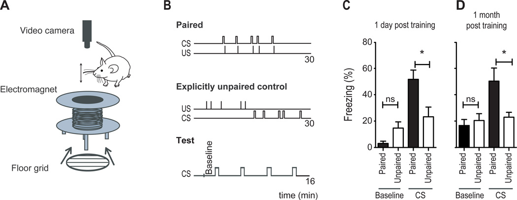
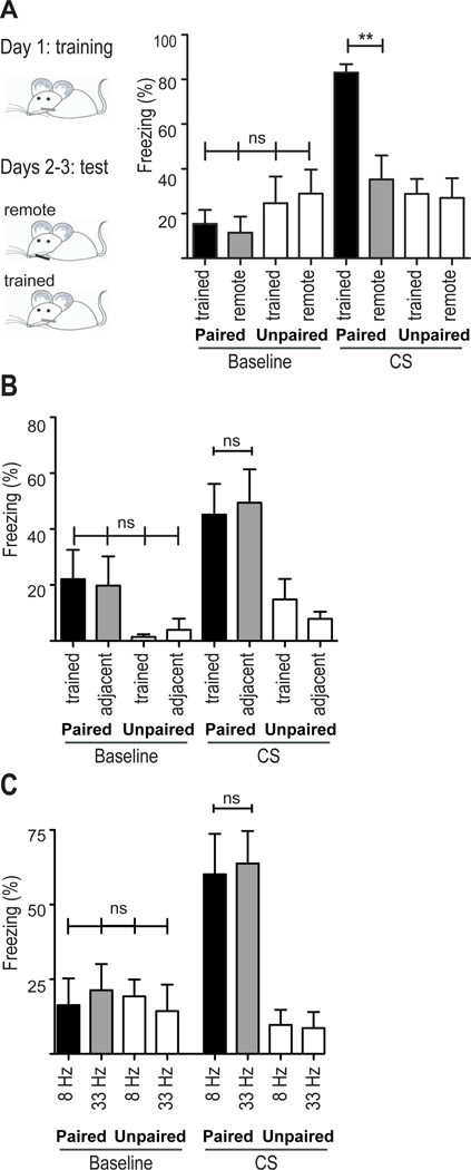
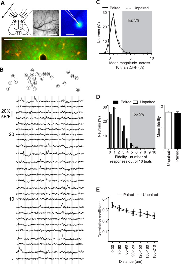
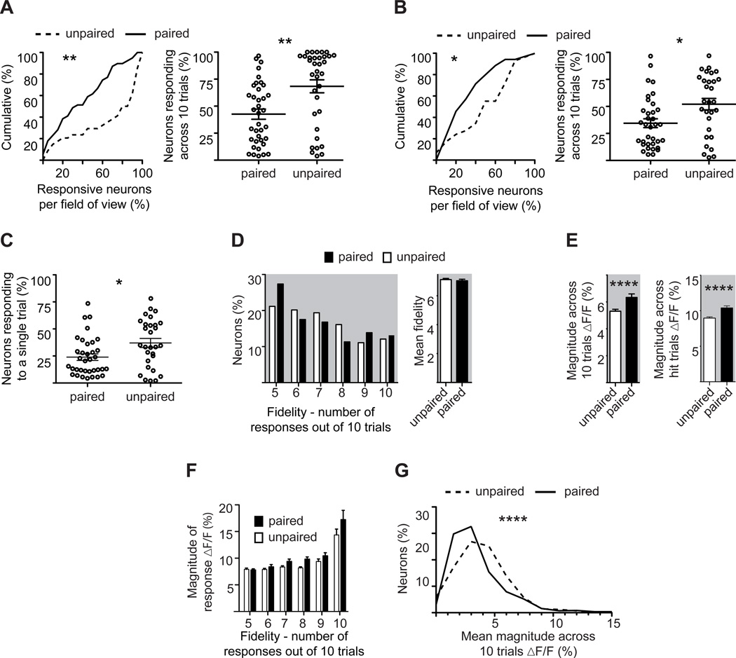
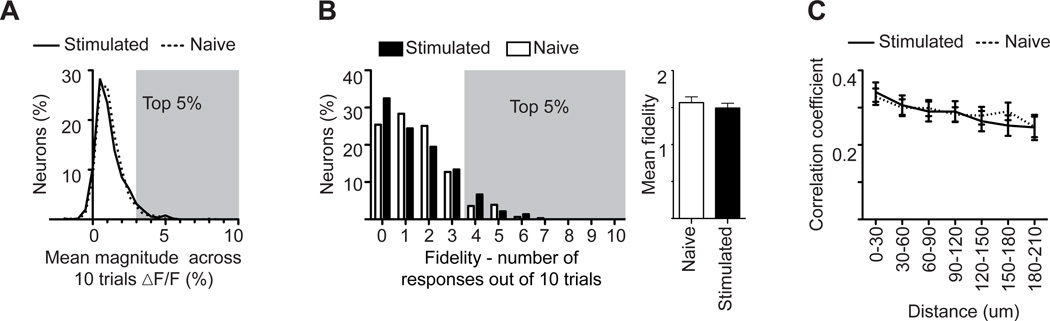
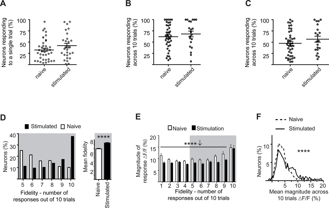
Several models of associative learning predict that stimulus processing changes during association formation. How associative learning reconfigures neural circuits in primary sensory cortex to "learn" associative attributes of a stimulus remains unknown. Using 2-photon in vivo calcium imaging to measure responses of networks of neurons in primary somatosensory cortex, we discovered that associative fear learning, in which whisker stimulation is paired with foot shock, enhances sparse population coding and robustness of the conditional stimulus, yet decreases total network activity. Fewer cortical neurons responded to stimulation of the trained whisker than in controls, yet their response strength was enhanced. These responses were not observed in mice exposed to a nonassociative learning procedure. Our results define how the cortical representation of a sensory stimulus is shaped by associative fear learning. These changes are proposed to enhance efficient sensory processing after associative learning.

Figure 1. Fear conditioning by passive whisker stimulation

(A) Schematic diagram showing the electromagnet used to passively deflect a whisker, the floor grid used to deliver foot-shock, and the camera used to track movement using FreezeFrame software. The mouse would be placed inside the bore of the magnet. (B) Schematic diagram showing the order and timing of the CS and US in paired and unpaired training procedures and at the time of testing. (C–D) Measurements of freezing in paired (black bars) and unpaired (open bars) conditioned mice during baseline and during CS, taken 1 day (C) or 1 month (D) after training; (ns non significant, *P<0.05, **P<0.01, ***P<0.001 Statistical analysis Student's t-test. Plots are mean ±SEM).

Figure 2. Measures of fear generalization

A,B. Mice were exposed to five foot shocks that were either paired or explicitly unpaired with whisker stimulation. A. The following two days the same mice were tested twice, one day on the trained whisker (black bars) and the next on a remote, untrained whisker (gray bars). The order of testing was randomized such that half were tested on the first day using the trained whisker and the other half using the remote whisker. Note the absence of generalization to the remote, untrained whisker. B. The same training paradigm as in (A) was used, but mice were tested on an adjacent, untrained whisker (gray bars). Note the generalization of the fear response to stimulation of the adjacent whisker. C. Mice were trained as in (A) and tested on the trained whisker twice: at the trained frequency (8 Hz; black bars) and a remote frequency (33 Hz; gray bars). Note the generalization of the fear response to the higher stimulation frequency. ns: non significant, **P<0.01. Statistical analysis: 1-way ANOVA followed by Tukey's post-hoc test. Plots are mean ±SEM.

Figure 3. Spontaneous activity is unchanged by associative fear learning

A. Intrinsic-signal imaging was used to identify the trained barrel and vascular landmarks were used to guide OGB-1 loading. An example image of the pial vasculature (top middle) and intrinsic response (top right) are shown. A typical image of labeled cortical neurons, imaged in vivo with 2-photon excitation, is shown in the lower panel. OGB-1 labeling is green; SR101 labeling, which labels astrocytes, is red and the overlap is yellow. Scale bars: Vascular and intrinsic maps, 500 µm; Calcium image, 50 µm. B. Example traces of spontaneous fluorescent changes in OGB-1 labeled neurons in layer 2/3. (Top) Each circle delineates a single neuron in the image in panel A. Each neuron is assigned a number. (Bottom) Change in fluorescence for each of the 26 cells identified above. The vertical gray lines indicate the timing of each sham whisker stimulation. Each trace is 120 seconds. C. Percentage of neurons as a function of mean magnitude of fluorescent change time-locked to a sham stimulus; dashed line indicates unpaired mice, solid line indicates paired mice. D. (Left) Percent of neurons as a function of their fidelity - the number of times their spontaneous activity was time locked to the sham stimuli. (Right) Mean fidelity of spontaneous events for each group averaged across all 10 sham stimuli. White bars indicate unpaired mice, black bars indicate paired mice. Gray shadings in C and D delineate the top 5% of neurons whose spontaneous activity was time locked to a sham stimulus. This was subsequently used as a threshold to define evoked responsive neurons with 95% confidence. E. Correlation coefficient of spontaneous activity between neurons as a function of the distance between them; dashed line indicates unpaired mice, solid line indicates paired mice. Note, the lack of a significant difference in C–E. Statistical analysis C,D, Mann-Whitney test; E 2-way ANOVA.

Figure 4. Example of evoked responses

A typical image of labeled cortical neurons, imaged in vivo with 2-photon excitation. OGB-1 labeling is green; SR101 labeling, which labels astrocytes, is red and the overlap is yellow. Scale bar: 50 µm. The numbered circles below the image identify each of the neurons whose responses are shown. The numbers in the circles correspond to the numbered traces (cells 1, 10, and 20 are labeled to the left of the traces). The vertical gray lines delineate the time of whisker stimulation. Each trace is 120 seconds.

Figure 5. Associative fear learning increases both sparse population coding and response strength

A. (Left) Cumulative percent of responding neurons across trials per field of view in paired (solid line) or unpaired (dashed line) mice. Responsive neurons were defined based on mean fluorescent change across 10 trials. (Right) Fractional response per field of view in paired and unpaired mice. Note the decreased fractional response after learning. B. As in (A), but defining responsive neurons based on fidelity. C. Percent of responsive neurons to a single stimulus trial per field of view in paired and unpaired mice. D. Percent of responding neurons (defined as in (B)) plotted as a function of fidelity (left), and averaged fidelity (right). Note the absence of any significant change between paired (black bars) and unpaired (white bars) mice. E. Mean fluorescence change of responding neurons measured in unpaired (white bars) and paired (black bars) mice across all 10 trials (left) or exclusive of failures (right). Note the significant increase in the paired group. F. Mean response magnitude as a function of fidelity, exclusive of failures, for responsive neurons in paired (black bars) or unpaired (white bars) mice. G. Percent of neurons, responsive and not, plotted as a function of their mean response magnitude, inclusive of failures, for paired (solid line) and unpaired (dashed line) mice. Note the reduction in the paired group. (*P<0.05, **<0.01, ***P<0.001, ****P<0.0001. Statistical analysis, A–G: Mann-Whitney test). Plots are mean ±SEM.

Figure 6. Spontaneous activity is unchanged by non-associative learning

A. Percentage of neurons as a function of mean magnitude of fluorescent change time-locked to a sham stimulus. Dashed line indicates naive mice, solid line indicates whisker stimulated mice. B. (Left) Percent of neurons as a function of their fidelity - the number of times their spontaneous activity was time locked to the sham stimuli. (Right) Mean fidelity for each group. White bars indicate naive mice, black bars indicate stimulated mice. Gray shadings in A and B delineate the top 5% of neurons whose spontaneous activity was time locked to a sham stimulus. This was subsequently used as a threshold to define evoked responsive neurons with 95% confidence. C. Correlation coefficient between neurons as a function of the distance between them; dashed line indicates naive mice, solid line indicates whisker stimulated mice. Note, the lack of a significant difference in A–C (Statistical analysis A–B: Mann-Whitney test; C: 2-way ANOVA). Plots are mean ±SEM.

Figure 7. Effects of non-associative training on cortical network responses

A. Percent of responsive neurons to a single stimulus trial per field of view in stimulated and naive mice. Note the absence of any significant change between the two groups. B. Fraction of neurons in each field of view responding across 10 stimulation epochs. Neurons were scored as responsive based on change in fluorescence across 10 trials. Note the absence of any significant difference between the two groups. C. Fraction of neurons in each field of view responding across 10 stimulation epochs. Neurons were scored as responsive based on response fidelity across 10 trials. Note the absence of any significant difference between the two groups. D. Percent of responding neurons (defined as in panel C) plotted as a function of their fidelity (left), and their averaged fidelity (right). Note the increase in fidelity in the stimulated group. E. Mean response magnitude as a function of fidelity, exclusive of failures, for all neurons in stimulated (black bars) or naive (white bars) mice. Note the lower magnitude in the stimulated group across fidelities 1–9. F. Percent of neurons, responsive and not, plotted as a function of their mean response magnitude, inclusive of failures, for stimulated (solid line) and naïve (dashed line) mice. Note the reduction in the naive group. (*P<0.05, **<0.01, ***P<0.001, ****P<0.0001; Statistical analysis, A–F: Mann-Whitney test). Plots are mean ±SEM.

References

1. Attwell D, Laughlin SB. An energy budget for signaling in the grey matter of the brain. J Cereb Blood Flow Metab. 2001;21:1133–1145. - PubMed
1. Bakin JS, Weinberger NM. Induction of a physiological memory in the cerebral cortex by stimulation of the nucleus basalis. Proc Natl Acad Sci U S A. 1996;93:11219–11224. - PMC - PubMed
1. Bao S, Chan VT, Merzenich MM. Cortical remodelling induced by activity of ventral tegmental dopamine neurons. Nature. 2001;412:79–83. - PubMed
1. Berlau KM, Weinberger NM. Learning strategy determines auditory cortical plasticity. Neurobiol Learn Mem. 2008;89:153–166. - PMC - PubMed
1. Bieszczad KM, Weinberger NM. Remodeling the cortex in memory: Increased use of a learning strategy increases the representational area of relevant acoustic cues. Neurobiol Learn Mem. 2010 - PMC - PubMed
Publication types
LinkOut - more resources