DynPeak: an algorithm for pulse detection and frequency analysis in hormonal time series

Abstract

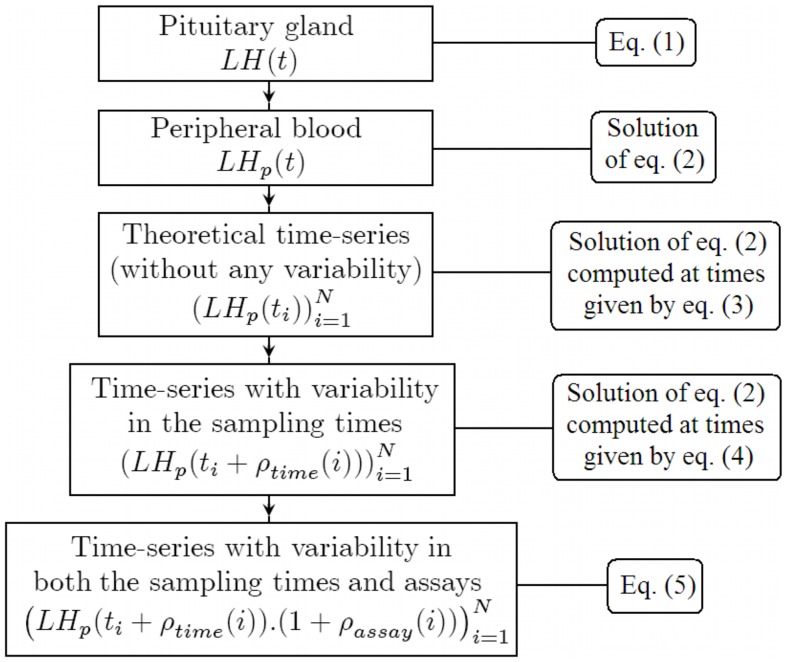
The endocrine control of the reproductive function is often studied from the analysis of luteinizing hormone (LH) pulsatile secretion by the pituitary gland. Whereas measurements in the cavernous sinus cumulate anatomical and technical difficulties, LH levels can be easily assessed from jugular blood. However, plasma levels result from a convolution process due to clearance effects when LH enters the general circulation. Simultaneous measurements comparing LH levels in the cavernous sinus and jugular blood have revealed clear differences in the pulse shape, the amplitude and the baseline. Besides, experimental sampling occurs at a relatively low frequency (typically every 10 min) with respect to LH highest frequency release (one pulse per hour) and the resulting LH measurements are noised by both experimental and assay errors. As a result, the pattern of plasma LH may be not so clearly pulsatile. Yet, reliable information on the InterPulse Intervals (IPI) is a prerequisite to study precisely the steroid feedback exerted on the pituitary level. Hence, there is a real need for robust IPI detection algorithms. In this article, we present an algorithm for the monitoring of LH pulse frequency, basing ourselves both on the available endocrinological knowledge on LH pulse (shape and duration with respect to the frequency regime) and synthetic LH data generated by a simple model. We make use of synthetic data to make clear some basic notions underlying our algorithmic choices. We focus on explaining how the process of sampling affects drastically the original pattern of secretion, and especially the amplitude of the detectable pulses. We then describe the algorithm in details and perform it on different sets of both synthetic and experimental LH time series. We further comment on how to diagnose possible outliers from the series of IPIs which is the main output of the algorithm.

Figure 1. Diagram of the synthetic sampling process.

Figure 2. Computation of a synthetic sample.

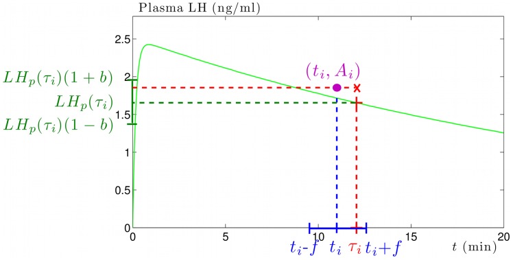
Solution LHp(t) of equation (2) (green curve), retained sampling time (blue dotted line), real sampling time (red dotted line) randomly chosen in (blue interval), exact value of LH level at time (green dotted line), retrieved LH level (red dotted line) randomly chosen in (green interval). The output of the i-th step of the sampling process is the couple (magenta disc) of time and corresponding LH level.

Figure 3. Effect of the variability of the sampling times upon the synthetic time series.

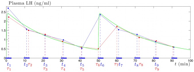
The , are the effective sampling times leading to the red-colored LH time series. The , are the expected sampling times leading to the blue-colored LH time series. The original, non-sampled time series corresponds to the green line. One can observe an instance of great discrepancy between the LH level measured at time , which corresponds to the very beginning of the ascending part of a pulse, and the LH level measured at time , which corresponds to the maximum of the same pulse.

Figure 4. Definition of pulse properties in the theoretical case versus experimental case.

For a theoretical pulse (i.e. a local maximum in the LHp(t) signal triggered by a spike in LH(t), we call “pulse time” the time at which LHp(t) admits a local maximum and “theoretical pulse amplitude” the value of LHp at this time. In a time series (either obtained from simulation and synthetic sampling protocol or experimental data), we call “pulse occurrence”, the time at which the time series admits a local maximum and “pulse amplitude” the corresponding value. Both the time values and the amplitude values are different in the theoretical and the experimental cases.

Figure 5. Effect of the sampling process upon a LH level signal with constant amplitude and pulse frequency.

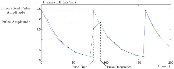
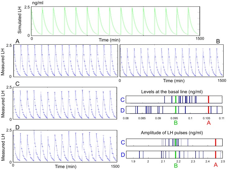
In all panels, . Top panel: theoretical continuously measured LH blood level (green curve). Panels A, B, C, D: sampling points (blue stars) of the time series obtained from the top panel signal through the sampling protocol. Panel A: first sampling time at r = 1 min, without any variability in the sampling process. Panel B: first sampling time at r = 4 min, without any variability in the sampling process. Panel C: first sampling time at r = 4 min, with variability in the sampling times . Panel D: first sampling time at r = 4 min, with variability both in the sampling times and the assays . The histograms correspond to the distribution of the levels at the basal line and the distribution of the amplitudes of the LH pulses, measured from the four cases A to D. The A and B time series, that only differ in the first sampling time, display constant (yet different) pulse amplitude. Red bars stand for case A (r = 1 min) value of the pulse amplitude (2.425 ng/ml) and level at the basal line (0.107 ng/ml). Green bars stand for case B (r = 4 min) value of the pulse amplitude (2.188 ng/ml) and level at the basal line (0.096 ng/ml). Blue bars stand for distributions of levels at the basal line and pulse amplitudes in case C (r = 4 min; f = 1.5 min) and case D (r = 4 min; f = 1.5 min; b = 10%, i.e. a variability of in the LH assays). In case D, the distributions of basal line levels (between 0.082 and 0.108 ng/ml) and pulse amplitudes (between 1.940 and 2.486 ng/ml) are wider than in case C (levels at the basal line between 0.092 and 0.101 ng/ml; pulse amplitude between 2.092 and 2.266 ng/ml), due to combined variabilities in the sampling times and assays.

Figure 6. Effect of the sampling process upon a LH level signal with regular increasing sampling frequency.

Case E (left panels): the pulse amplitude remains almost constant and the basal line increases regularly. Case F (right panels): the pulse amplitude decreases regularly and the basal line decreases regularly. Panels on row 1 represent the fine step simulation of LH blood level. Histograms on row 2 display the distribution of the LH pulse amplitudes and the distribution of the levels at the basal line, measured from the two theoretical LH level signals shown in row 1. A zoom on the distribution of the pulse amplitudes is shown as an insert in case E. Panels on row 3 represent the time series (blue stars) along the theoretical continuously measured LH level (green curve). Panels on row 4 represent the resulting LH measured time series (measured LH levels versus sampling times linked with segments). In both cases E and F, the sampling period is Ts = 10 min. In case E, the initial sampling time occurs at the first minute of the simulation (r = 1 min), without any variability in the sampling times (f = 0 min) or the assays (b = 0%). In case F, the initial sampling time occurs at the fourth minute of the simulation (r = 4 min), with variability both in the sampling times (f = 2 min) and the assays (b = 5%). Histograms on row 5 display the distribution of the LH pulse amplitudes and the distribution of the LH levels at the basal line, measured from the time series shown in row 4. While the distributions are regular in the theoretical time series, they become completely irregular in the sampled time series. As a result, the range of amplitudes is shortened. Regarding the distribution of the levels at the basal line, it is worth noticing that the measured values (E: between 0.125 and 0.519 ng/ml; F: between 0.094 and 0.258 ng/ml) are greater than the theoretical values (E: between 0.098 and 0.434 ng/ml; F: between 0.075 and 0.171 ng/ml). On the contrary, in case E, it is worth noticing that the theoretical pulse amplitudes vary from 2.379 to 2.425 ng/ml whereas measured pulse amplitudes vary from 1.447 to 2.395 ng/ml. In case F, all measured pulse amplitudes (between 0.302 and 1.959 ng/ml) are lower than the corresponding theoretical values (between 0.353 and 2.315 ng/ml).

Figure 7. IPI series from synthetic LH time series with different sampling frequencies.

Left panels: LH plasma level time series retrieved over 1000 min. Vertical lines correspond to the pulse occurrences. Panel A: theoretical plasma level, corresponding to a continuous monitoring. The pulse frequency increases, whereas the pulse amplitude decreases along time. Panels B, C and D: sampled series, with a respective sampling period of 1, 5 or 10 min. Stars on the time series correspond to sampled points. The first sampling time occurs at the first minute of the simulation (r = 1 min), variability in the sampling times is set to 15% of the sampling period (f = 0.15 min for B, f = 0.75 min for C and f = 1.5 min for D) and the assay variability is set to b = 5%. Right panels: resulting IPI series, indexed by the number of the pulse occurrence (each IPI is represented by a black diamond). The theoretical IPI series is the continuous green curve, superimposed on the IPI series obtained after sampling. In any case, there are 16 detected peaks.

Figure 8. IPI series from experimental LH series with different pulsatile rhythms.

Left panels: LH plasma level time series with a 10 min. sampling period. Vertical lines correspond to the pulse occurrences. Stars on the time series correspond to sampled points. Right panels: resulting IPI series (black diamond), indexed by the number of the pulse occurrence. Panel A: stable rhythm with final acceleration. Panel B: progressive acceleration. Panel C: fast deceleration in the second half of the series.

Figure 9. IPI outliers lying above the upper bound of the tunnel. Example of correction by decreasing the value of the relative magnitude threshold, .

Top panels: two experimental LH plasma time series, A (panels A1 and A2) and B (panel B). Vertical lines correspond to pulse occurrences. Bottom panels: resulting IPI series indexed by time. Each IPI value (blue point) corresponds to the time elapsed between the current detected pulse and the previous one. Dashed line: moving cubic function fitting the values of the IPI series. Solid lines: lower (-dependent function ) and upper (-dependent function ) edges of the tunnel (). 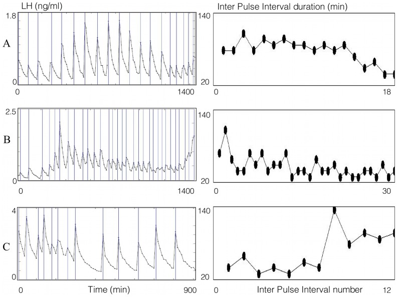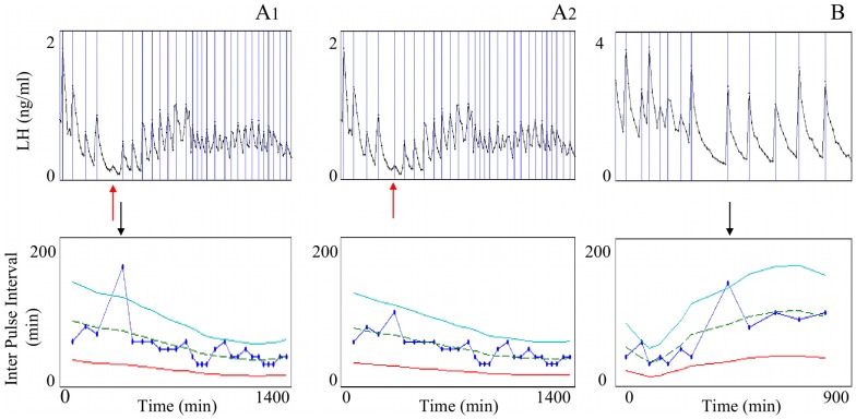Black arrows: occurrences of the outliers. Case A: outlier due to a lack of detection (missed pulse designed by a red arrow); panel A1: initial IPI series with (default value); A2: corrected IPI series; with . Case B: genuine long IPI.

Figure 10. IPI outliers lying below the lower bound of the tunnel. Example of correction by increasing the value of the relative magnitude threshold, .

Top panels: two experimental LH plasma time series, A (panel A) and B (panels B1 and B2). Bottom panels: resulting IPI series indexed by time. The vertical lines, the blue points, the dashed line and the solid lines represent the same objects as in Figure 9. Panels A and B1: initial IPI time series. Solid black arrows: occurrence of clear outliers. Dashed black arrows: occurrence of IPIs that can be associated with over-detected peaks in the LH series although they remain above the lower bound of the tunnel. Red arrows: peaks lying on the middle of the descending phase of the preceding pulse. Green arrow: peak lying on the middle of the ascending phase of the following pulse. 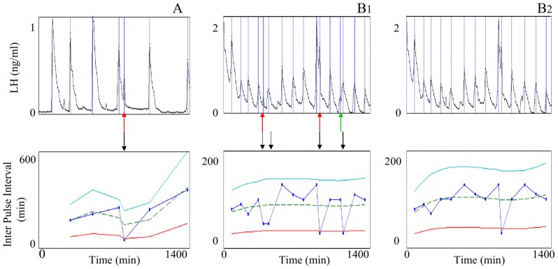Panel B2: B corrected IPI series after increasing the relative magnitude threshold to 0.45. Two of the three false peaks have been discarded.

Figure 11. IPI-based study of the synchronization between LH series.

The four LH series are retrieved from ewes subject to an experimental protocol inducing a steep decrease in the pulse frequency. Left panels: experimental LH plasma time series; vertical lines correspond to pulse occurrences. Right panels: resulting IPI series indexed by time. The vertical lines, the dashed line and the solid lines represent the same objects as in Figure 9. Vertical dashed line: break in the dynamics of the IPI series corresponding to the last IPI preceding the outlier.

References

-
- Sollenberger M, Carlsen E, Johnson M, Veldhuis J, Evans W. Specific Physiological Regulation of Luteinizing Hormone Secretory Events Throughout the Human Menstrual Cycle: New Insights into the Pulsatile Mode of Gonadotropin Release. J Neuroendocrinol 6. 1990;(2):845–852. - PubMed
- Moenter S, Caraty A, Karsch F. The estradiol-induced surge of gonadotropin-releasing hormone in the ewe. Endocrinology. 1990;127:1375–1384. - PubMed
- Moenter S, Brand R, Karsch F. Dynamics of gonadotropin-releasing hormone (GnRH) secre- tion during the GnRH surge: insights into the mechanism of GnRH surge induction. Endocrinology. 1992;130:2978–2984. - PubMed
- Clarke I, Moore L, Veldhuis J. Intensive direct cavernous sinus sampling identifies high-frequency, nearly random patterns of FSH secretion in ovariectomized ewes: combined appraisal by RIA and bioassay. Endocrinology 143. 2002;(1):117–129. - PubMed
- Drouilhet L, Taragnat C, Fontaine J, Duittoz A, Mulsant P, et al. Endocrine Characterization of the Reproductive Axis in Highly Prolific Lacaune Sheep Homozygous for the FecLL Mutation. Biol Reprod 82. 2010;(5):815–824. - PubMed
Publication types
MeSH terms
Substances
LinkOut - more resources
Full Text Sources
Other Literature Sources
Research Materials