Visuomotor functional network topology predicts upcoming tasks

Abstract

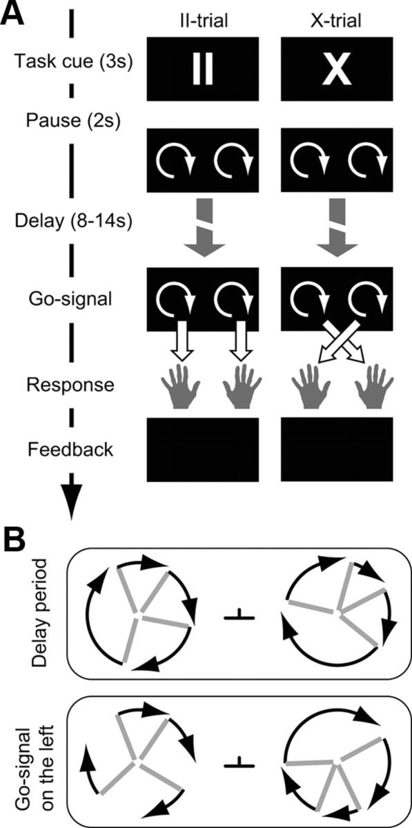
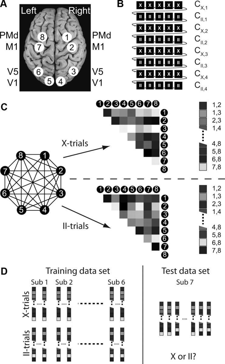
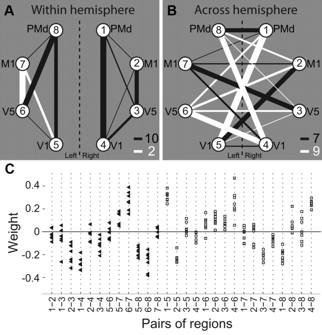
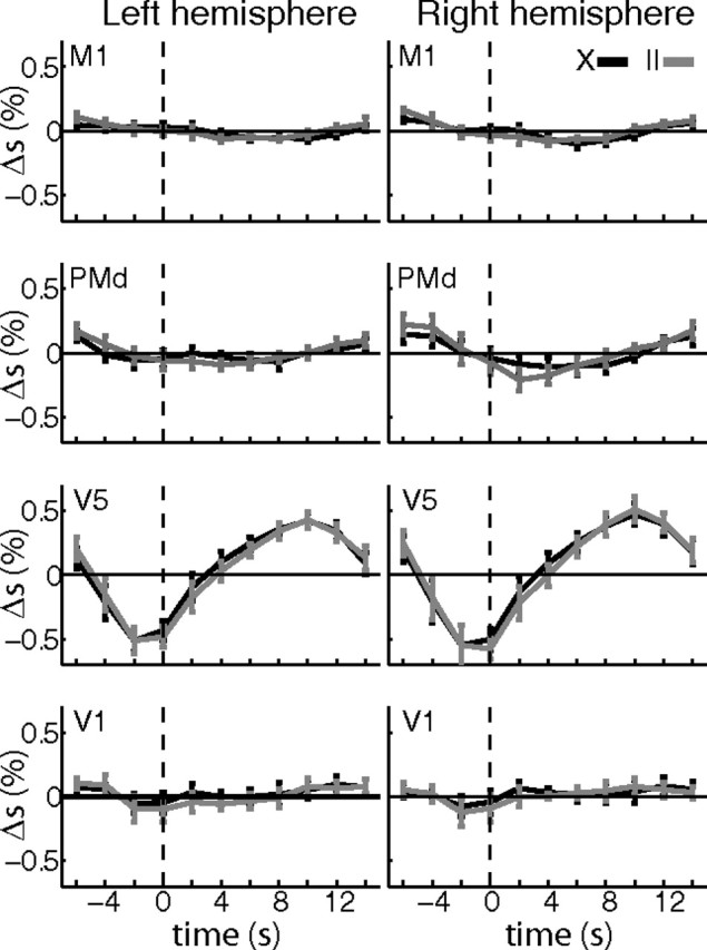
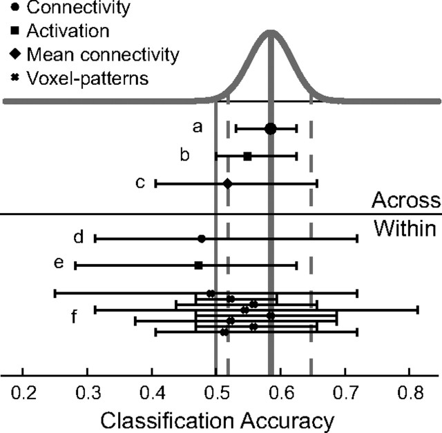
It is a vital ability of humans to flexibly adapt their behavior to different environmental situations. Constantly, the rules for our sensory-to-motor mappings need to be adapted to the current task demands. For example, the same sensory input might require two different motor responses depending on the actual situation. How does the brain prepare for such different responses? It has been suggested that the functional connections within cortex are biased according to the present rule to guide the flow of information in accordance with the required sensory-to-motor mapping. Here, we investigated with fMRI whether task settings might indeed change the functional connectivity structure in a large-scale brain network. Subjects performed a visuomotor response task that required an interaction between visual and motor cortex: either within each hemisphere or across the two hemispheres of the brain depending on the task condition. A multivariate analysis on the functional connectivity graph of a cortical visuomotor network revealed that the functional integration, i.e., the connectivity structure, is altered according to the task condition already during a preparatory period before the visual cue and the actual movement. Our results show that the topology of connection weights within a single network changes according to and thus predicts the upcoming task. This suggests that the human brain prepares to respond in different conditions by altering its large scale functional connectivity structure even before an action is required.

Figure 1.

Visuomotor mapping task. A, Time line of a single pro-trial (II, left) and anti-trial (X, right). At the beginning of each trial, the task cue II or X was shown. During an extended delay period (between 8 and 14 s), the subject viewed two rotating clocks and tried to detect the go-signal (when one of the two clocks synchronized its hands; B). During this delay period, the connectivity in the visuomotor network was assessed. B, During the delay period, all clock hands (gray) turned with different velocities. At the go-signal, the hands of one clock synchronized. The black arrows indicate the velocities and were not displayed in the paradigm. For clarity, only four hands per clock are depicted. In the experiment, each clock consisted of eight hands. During the whole experiment, subjects had to fixate on the fixation spot between the two clocks.

Figure 2.

Regions of interest and connectivity graph classification procedure. A, The eight (4 per hemisphere) ROIs are illustrated. B, Illustration of run structure and assignment of data. The two task conditions were presented in miniblocks of five trials. Trials are drawn as black boxes (X, anti-trials; II, pro-trials). Gray arrows indicate the sequence of trials during one run. Note that only a part of one run is shown. All consecutive trials of one miniblock, i.e., one row, were assigned to one subset (without the catch trial) from which the correlation matrix C was computed (e.g., C_X,1 is the correlation matrix for the first subset of the contralateral condition). C, The eight ROIs form a fully connected graph (left). The connectivity structure, i.e., correlation matrix, is calculated for all II and X miniblocks and transformed to vectors of all connections (right), which are then used for the multivariate analysis. Note that the elements on the diagonal of the correlation matrix and the lower half remained empty because of the symmetry of the correlation structure. D, The connectivity vectors of all miniblocks of six subjects were used to train a support vector classifier to distinguish between the connection graphs for the II and the X blocks. The classifier was then tested on the connectivity data from the seventh subject.

Figure 3.

Behavioral results. A, Left, Average number of correct trials per miniblock for individual subjects. Short catch trials were not counted. Therefore, there were four trials per block. Right, Percentage of correct trials averaged over subjects. B, Left, Average reaction time for individual subjects. The average and SD were calculated over all correct trials of each individual subject. Right, Group average of reaction times. Black bars, X trials; white bars, II trials. Error bars show the SD.

Figure 4.

Activation differences during delay period. The activations (p < 0.001, k = 10) of the II versus X (X vs II) contrast were used to create masks and extract the percentage signal change (Δs) in these regions. The masks consisted of a sphere with a volume of 57 voxels (radius, 7 mm) around the peak activation. Average activations (percentage signal change, Δs) are shown for the four regions that showed a significant difference at p < 0.001 (uncorrected, k = 10) between II and X trials. All correct trials of a condition were temporally aligned to the onset of the delay period (dashed vertical line) and then averaged over subjects (n = 7). Average traces of percentage signal change are shown for X trials (black) and II trials (gray). Error bars are SEM. Note that none of the small differences between the two task conditions survived a Bonferroni correction for multiple time points (n = 11). Nevertheless, when fitted with the regressors defined in the GLM, these four regions showed a significant activation. This difference could arise because the GLM regressors take into account the length of the delay period. FG, Right fusiform gyrus; IOG, right inferior occipital gyrus; BS, brainstem; SFG, left superior frontal gyrus.

Figure 5.

Discriminative weight structure of classifier. A, B, The weights of the support vector classifier are depicted for all connections within hemisphere (A) and between hemispheres (B) for the network of eight ROIs. The nodes of the graph correspond to the ROIs (compare Fig. 2). The line thickness is proportional to the absolute value of the respective dimension of the average weight vector. Hence, it is related to the amount of information about the two conditions that is present in the temporal correlation between the respective region pair. The line color gives information of the sign of the weight corresponding to the connection (black, minus; white, plus). Numbers at the bottom right of A and B indicate the number of black and white lines in the two graphs. The number of black lines in A, and thus, the number of white lines in B, are significantly higher than expected by chance (p = 0.04). C, Illustration of weights versus connections for all cross-folds individually. For every connection (x-axis), the corresponding weight is plotted for all seven cross-folds. Black triangles depict intrahemispheric connections; white squares are interhemispheric connections. Connections are ordered to confirm with A and B: intrahemispheric connections on the left, interhemispheric connections on the right.

Figure 6.

Average activation in visuomotor network. Average activations (percentage signal change, Δs) are shown for the eight regions of the visuomotor network. Normalized (MNI) masks of the eight ROIs were calculated for this purpose. Specifically, we normalized the individual masks of each subject to the MNI template and then selected for each ROI the 50 voxels with the highest overlap between the masks of all seven subjects. The normalized masks were used to extract average time courses from the normalized and smoothed data. Correct trials of a condition were temporally aligned at the onset of the rotating clocks (dashed vertical line) and then averaged over subjects (n = 7). Average traces of percentage signal change (black, X trials; gray, II trials) are shown for the eight regions of the visuomotor network (legend on top right). Error bars show SEM. A sign rank test at a liberal threshold of p < 0.05 yielded only few significant differences in percentage signal change (Δs) between X and II trials, none of which survived a correction for multiple comparisons for the number of time points (Bonferroni, n = 11). Please note that the average traces contain left and right button presses and are aligned to the onset of the visual stimulus and not to the motor response. Hence, motor-related BOLD activity as confirmed by the GLM control analysis is averaged out and cannot be seen here.

Figure 7.

Illustration of different classification schemes. The results of all feature selection and cross-validation schemes used in this study are illustrated. The Beta-distribution, Beta (n_c + 1, n_e + 1), that describes the result of the classifier of the main analysis is plotted on top (gray curve). The average accuracy (solid gray; 58.5%) and the 95% confidence interval (dashed gray; 51.9% and 64.8%) are shown as vertical lines. Chance level (50%) is indicated by the thin vertical solid gray line. Different feature selection methods are indicated by a symbol (key in top left) showing the average accuracy across subjects. Each classifier is further characterized by a horizontal line indicating the full range observed, i.e., from minimum to maximum within-subject accuracy. a, Classification across subjects on connectivity graphs (main analysis). b, Classification across subjects on ROI activation. c, Classification across subjects on average within versus between connectivity. d, Classification within subjects on connectivity graphs. e, Classification within subjects on ROI activation. f, Classification within subjects on voxel pattern within ROIs. In f, ROIs are (from top to bottom): right PMd, right M1, right V5, right V1, left V1, left V5, left M1, and left PMd (compare Fig. 2). Note the large variability in the within-subject classifiers, which might be due to the small number of training samples compared with across-subject classification. It is important to note that it was not the goal of this study to maximize the classification accuracy but to test classification across subjects based on connectivity graphs.

References

1. Alemán-Gómez Y, Melie-García L, Valdés-Hernandez P. IBASPM: toolbox for automatic parcellation of brain structures. Paper presented at 12th annual meeting of the Organization for Human Brain Mapping; Florence, Italy. 2006.
1. Bishop CM. Pattern recognition and machine learning (information science and statistics) New York: Springer; 2006.
1. Bode S, Haynes JD. Decoding sequential stages of task preparation in the human brain. Neuroimage. 2009;45:606–613. - PubMed
1. Brass M, von Cramon DY. The role of the frontal cortex in task preparation. Cereb Cortex. 2002;12:908–914. - PubMed
1. Brodersen KH, Schofield TM, Leff AP, Ong CS, Lomakina EI, Buhmann JM, Stephan KE. Generative embedding for model-based classification of fMRI data. PLoS Comput Biol. 2011;7:e1002079. - PMC - PubMed
Publication types
LinkOut - more resources