Interactive semiautomatic contour delineation using statistical conditional random fields framework

Abstract

Purpose: Contouring a normal anatomical structure during radiation treatment planning requires significant time and effort. The authors present a fast and accurate semiautomatic contour delineation method to reduce the time and effort required of expert users.

Methods: Following an initial segmentation on one CT slice, the user marks the target organ and nontarget pixels with a few simple brush strokes. The algorithm calculates statistics from this information that, in turn, determines the parameters of an energy function containing both boundary and regional components. The method uses a conditional random field graphical model to define the energy function to be minimized for obtaining an estimated optimal segmentation, and a graph partition algorithm to efficiently solve the energy function minimization. Organ boundary statistics are estimated from the segmentation and propagated to subsequent images; regional statistics are estimated from the simple brush strokes that are either propagated or redrawn as needed on subsequent images. This greatly reduces the user input needed and speeds up segmentations. The proposed method can be further accelerated with graph-based interpolation of alternating slices in place of user-guided segmentation. CT images from phantom and patients were used to evaluate this method. The authors determined the sensitivity and specificity of organ segmentations using physician-drawn contours as ground truth, as well as the predicted-to-ground truth surface distances. Finally, three physicians evaluated the contours for subjective acceptability. Interobserver and intraobserver analysis was also performed and Bland-Altman plots were used to evaluate agreement.

Results: Liver and kidney segmentations in patient volumetric CT images show that boundary samples provided on a single CT slice can be reused through the entire 3D stack of images to obtain accurate segmentation. In liver, our method has better sensitivity and specificity (0.925 and 0.995) than region growing (0.897 and 0.995) and level set methods (0.912 and 0.985) as well as shorter mean predicted-to-ground truth distance (2.13 mm) compared to regional growing (4.58 mm) and level set methods (8.55 mm and 4.74 mm). Similar results are observed in kidney segmentation. Physician evaluation of ten liver cases showed that 83% of contours did not need any modification, while 6% of contours needed modifications as assessed by two or more evaluators. In interobserver and intraobserver analysis, Bland-Altman plots showed our method to have better repeatability than the manual method while the delineation time was 15% faster on average.

Conclusions: Our method achieves high accuracy in liver and kidney segmentation and considerably reduces the time and labor required for contour delineation. Since it extracts purely statistical information from the samples interactively specified by expert users, the method avoids heuristic assumptions commonly used by other methods. In addition, the method can be expanded to 3D directly without modification because the underlying graphical framework and graph partition optimization method fit naturally with the image grid structure.

Figure 1

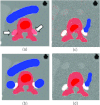
(a) Illustration of semiautomatic segmentation process. (b)The user uses brush strokes of one color to identify the target structure, liver in this case, and brush strokes of a different color for background. (c) Segmentation result is shown shaded so the user can review and modify the result with additional brush strokes. (d) The brush strokes are automatically carried over to subsequent slices until they are no longer applicable, at which point the user can redraw the brushes.

Figure 2

The edge cost assignment of the graph to solve the minimization of three different energy functions using min s-t cut. A non-negative weight (cost) is assigned to each edge. Min s-t cut is usually solved through a maximum flow algorithm. The arrow of an edge shows the direction of the flow. (a) Greig's energy function in Eq. 1 for image binary denoising. (b) Boykov's energy function in which a heuristic boundary term B_ij is defined in Eq. 2 for image segmentation. In addition, seed points for the classes, labeled h for target and j for nontarget, can be indicated by users. For those seed nodes, either a very large number K or zero is assigned to the cost of links to s and t to serve as hard constraints. (c) Our energy function, Eq. 3, derived from CRF, in which the probabilistic boundary term Eq. 5 is defined for image segmentation and is used for cost of edges connecting neighboring voxels. (d) An example of a minimum cut. Dashed lines indicate the edges being cut. The minimum cost of a cut to separate nodes 1, 2, and 3 into two separated groups is 2 + 4 + 8 + 2. After the cut, node 1 and 2 remain connected to s and are classified as target while node 3 remains connected to t and is classified as nontarget.

Figure 3

Graph-based interpolation. The solid line contours are segmented from our graph cut method on the two slices p and r. On the slice q being interpolated, the nodes in black do not need re-estimation since their adjacent nodes on slice p and r are assigned to the same class. Their edge costs are interpolated as Eq. 7 from slices p and r. The node in white needs re-estimation since its adjacent nodes on slice p and r are assigned to two different classes. A graph min-cut is then applied to the partially interpolated graph on slice q for segmentation.

Figure 4

Segmentation results from the phantom image. (a) On noise-free images, Boykov's boundary term favoring high contrast [Eq. 5] is prone to leakage if a high contrast boundary is present in nearby tissue (arrow). (b) Additional brush strokes are needed to exclude neighboring tissue. (c) On an image with 4% Gaussian noise, using Boykov's boundary term and strongly weighted regional term results in an irregular boundary and pixels within the segmentation are excluded. (d) In contrast, our method SAASS requires fewer brush strokes and preserves piece-wise continuity.

Figure 5

Liver segmentation of a patient. Typical image slices from superior to inferior are shown. Physician-drawn contours in dark gray and SAASS contours are in light gray.

Figure 6

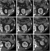
Kidney segmentation of a patient. Typical image slices from superior to inferior are shown. Physician-drawn contours in dark gray and SAASS contours are in light gray.

Figure 7

Comparison of liver segmentations: SAASS (dashed white), RG (black), MIPAV-LS (dark gray), and Seg3D-LS (light gray). RG, MIPAV-LS, and Seg3D-LS segmentations show leakage (arrows) since they are sensitive to low-contrast boundary and surrounding high contrast tissues.

Figure 8

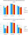
Overlay analysis for liver and kidney segmentation. SAASS has the best DSC and smallest variation among the four methods compared.

Figure 9

Mean Hausdorff distance comparison in ten liver cases and eight kidney cases. Error bars show the minimum and maximum distances over the cases.

Figure 10

Sensitivity, specificity, and DSC measures comparison between SAASS graph-based interpolation and mesh-based interpolation. Mean of the measures in five liver cases are shown.

Figure 11

(Top row) Image slices where liver topology changes. The light gray contours in the middle slice are interpolated from the dark gray contours in the adjacent slices on the left and right based on surface tiling method, but suffer from topological change. The pale gray contours are result of our graph-based interpolation method (Sec. 2E). (Bottom row) Even without topological change, our method still shows improved performance over surface tiling (middle), due the utilization of image information.

Figure 12

Bland–Altman plot of interobserver agreement in five kidney cases. Absolute value of the difference is used in y axis. SAASS shows better repeatability and the difference is irrelevant to the size of volumes.

Figure 13

Bland–Altman plots of intraobserver agreement for Observer 1 and Observer 2. In both observers, SAASS has better agreement compared to the manual method.

Figure 14

Comparison of performance of the manual method and SAASS. Mean time per slice for segmentations of five kidney cases is calculated from the two observers. The error bars show one standard deviation.

Figure 15

An example to demonstrate leakage. (a) The image shows blurred boundary between the liver left lobe and the apex of the heart. (b) Leakage of the initial segmentation due to blurred boundary. (c) An additional brush stroke to remove the leakage. The ground truth contour is shown.

Figure 16

Examples of segmentation on other organs and other modalities: (a) bladder and (b) heart in CT; (c) brainstem and (d) parotid in MR images. We note that MR inhomogeneity in pixel intensity should be corrected prior to intensity-based segmentation methods.

References

1. Fox J. L., Rosenzweig K. E., Rengan R., O’Meara W., Yorke E., Erdi Y., Nehmeh S., and Leibel S. A., “Does the registration of PET and planning CT images decrease inter-and intra-observer variation in delineating tumor volumes for non-small-cell lung cancer (NSCLC)?,” Int. J. Radiat. Oncol., Biol., Phys. 62, 70–75 (2005).10.1016/j.ijrobp.2004.09.020 - DOI - PubMed
1. Bae K. T., Giger M. I., Chen C. T., and Kahn C. E., “Automatic segmentation of liver structure in CT images,” Med. Phys. 20, 71–78 (1993).10.1118/1.597064 - DOI - PubMed
1. Gao L., Heath D. G., Kuszyk B. S., and Fishman E. K., “Automatic liver segmentation technique for three-dimensional visualization of CT data,” Radiology 201, 359–364 (1996). - PubMed
1. Adams R. and Bischof L., “Seeded region growing,” IEEE Trans. Pattern Anal. Mach. Intell. 16(6), 641–647 (1994).10.1109/34.295913 - DOI
1. Pohle R. and Toennies K. D., “Segmentation of medical images using adaptive region growing,” Proc. SPIE Med. Imaging: Image Process. 4322, 1337–1346 (2001).10.1117/12.431013 - DOI
Publication types