The neuroimaging signal is a linear sum of neurally distinct stimulus- and task-related components

Abstract

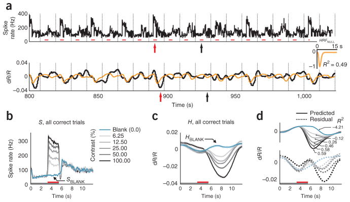
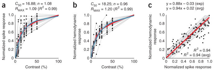
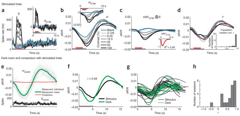
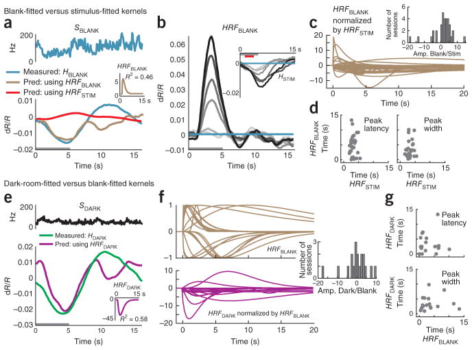
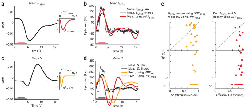
Neuroimaging (for example, functional magnetic resonance imaging) signals are taken as a uniform proxy for local neural activity. By simultaneously recording electrode and neuroimaging (intrinsic optical imaging) signals in alert, task-engaged macaque visual cortex, we recently observed a large anticipatory trial-related neuroimaging signal that was poorly related to local spiking or field potentials. We used these same techniques to study the interactions of this trial-related signal with stimulus-evoked responses over the full range of stimulus intensities, including total darkness. We found that the two signals could be separated, and added linearly over this full range. The stimulus-evoked component was related linearly to local spiking and, consequently, could be used to obtain precise and reliable estimates of local neural activity. The trial-related signal likely has a distinct neural mechanism, however, and failure to account for it properly could lead to substantial errors when estimating local neural spiking from the neuroimaging signal.

Figure 1

The full hemodynamic signal is poorly predicted by local multi-unit spiking. (a) Top, a section of the full recorded spiking signal (S) for a representative experimental session (black trace). Bottom, corresponding measured hemodynamic signal (H, black) and the best prediction obtained from spiking (orange, $H_{\text{NULL}}^{\text{PRED}}={\mathit{HRF}}_{\text{NULL}}\otimes S$, ⊗ indicates convolution; Supplementary Note, equation (3)). Inset, best fitting kernel HRF_NULL (amplitude normalized) obtained by fitting H to S. Mean R² = 0.49, as calculated using mean signals averaged across contrasts (n = 261 trials total, roughly 43 per contrast). Red line segments indicate stimulus application and vertical dotted lines indicate fixation trial onset. Red and black arrows below traces indicate typical responses to high-contrast (100% contrast) and blank (0% contrast) stimuli, respectively; for hemodynamics, increasing negative amplitudes, that is, increasing absorption of light by cortex, equals increasing blood volume. Note the poor match between the observed and predicted traces leading to a large residual and, consequently, low mean R². (b) Trial-aligned averages of spiking (S) for each contrast. The trial structure is indicated by the color bars (gray, fixate; red, stimulus; no bar, relax). Note the prominent blank-trial spiking signal S_BLANK. (c) Data presented as in b for hemodynamics (H). (d) Data are presented as in b for corresponding predicted hemodynamics $H_{\text{NULL}}^{\text{PRED}}$ (solid lines, top) and residuals ( $H-H_{\text{NULL}}^{\text{PRED}}$, dotted lines, bottom; separated vertically for visibility). Individual R², calculated separately per contrast, are shown alongside each prediction. Data were obtained from monkey S. Error bars represent s.e.m.

Figure 2

Results using the MLM: stimulus-evoked (blank subtracted) hemodynamic responses (H_STIM) are reliably and linearly predicted by stimulus-evoked local spiking (S_STIM). (a, b) S_STIM (a) and H_STIM (b) (shaded regions indicate integration windows for calculating mean response strength; see Fig. 3). Data are presented as in Figure 1 with error bars indicating s.e.m. The trial structure is indicated by the color bars (gray, fixate; red, stimulus; no bar, relax). (c) Predicted stimulus-evoked hemodynamics ( $H_{\text{STIM}}^{\text{PRED}}={\mathit{HRF}}_{\text{STIM}}\otimes S_{\text{STIM}}$; Supplementary Note, equation (8)) and corresponding R², contrast by contrast. Dotted traces indicate residuals ( $H_{\text{STIM}}-H_{\text{STIM}}^{\text{PRED}}$). Inset, optimal HRF_STIM (mean R² = 0.99, n = 261 trials). (d) Comparing mean R² for the null model, that is, without blank subtraction (y axis) against the MLM (x axis). Population average (s.e.m.) of mean R² = 0.93 (0.01) for MLM, 0.57 (0.05) for the null model (n = 34 sessions, 3 monkeys). (e) Data are presented as in d for R² calculated separately by contrast and then averaged (one data point per experiment). Fits for the null model were almost all worse than for the MLM (that is, below the diagonal) and included many negative values (shown below scatter plot; population average R² (s.e.m.): MLM, 0.77 (0.03); null model, 0.14 (0.10); n = 34). See Supplementary Figure 3 for bootstrap estimates of confidence intervals. (f) All HRF_STIM kernels (amplitude normalized; color coded by animal; population average latency (s.e.m), 3.1 (0.2) s; population average width (s.e.m.), 3.3 (0.2) s:, n = 34). Inset, average mean R² (s.e.m.) from cross-validation tests using leave-one-out mean kernels, over all animals (0.80 (0.03), n = 34) and separately by animal (monkey S, 0.89 (0.02), n = 17; monkey T, 0.85 (0.03), n = 15; monkey Y, 0.90 (0.01), n = 2). R² pop indicates experimental population average (data from d).

Figure 3

Stimulus-evoked spiking and hemodynamics are hyperbolic functions of stimulus contrast and are linearly related to each other. (a) Normalized stimulus-evoked spike responses across contrasts. Each point shows data for a single contrast on a given session, averaged over the integration window as shown in Figure 2a. Gray lines link sets of points in individual sessions. The red line (piecewise continuous) indicates the average across sessions. The blue line represents the optimal fitted hyperbolic response function R(C) of contrast C, of the form $R(C)=R_{max}\left(\frac{C^n}{C^n+C_{50}^n}\right)$; fitted parameters are shown above. (b) Data are presented as in a for stimulus-evoked hemodynamic responses, averaged over the window as in Figure 2b. (c) The spiking and hemodynamic responses shown in a and b, plotted against each other. The gray lines are regression lines for each session and the red line is the average of the regression lines. Expressions show regression and R², both for the experiments in Figures 1 and 2a–c (exp) and the population (avg). Population averages were calculated from session values, weighted by number of trials within a session (n = 34 sessions, 3 monkeys).

Figure 4

Estimated trial-related signal T is consistent across contrasts, across experiments, and between stimulated and dark-room trials. (a, b) Spiking (a) and hemodynamics (b) from another representative session. Insets, corresponding S_STIM and H_STIM. The trial structure is indicated by the color bars (gray, fixate; red, stimulus; no bar, relax). (c) Prediction convolving optimal kernel HRF_STIM (inset) with full spiking S (that is, HRF_STIM ⊗S). (d) Estimated trial-related signals (T =〈H −HRF_STIM ⊗ S〉; Supplementary Note, equation (9)) shown individually by contrast; red indicates mean across contrasts. Note the high amplitude of mean T (s.d. = 0.0088, compared with 0.0058 for H_STIM using 100% contrast; a 1.5-fold difference). Note the marked similarity of signals T across contrasts (correlation (Pearson’s r) with leave-one-out means: 0.99, 0.99, 0.99, 0.99, 0.99, 0.99 and 0.96 for contrasts 0–100% in sequence; n = 175 trials, 25 per contrast, 7 contrasts, median r = 0.99). Inset, population histogram of median r (mean (s.e.m.) = 0.94 (0.01), n = 34). (e) Dark-room trials for the sessions shown in a–d. Top, hemodynamic traces, H_DARK. Gray lines are individual traces, all correct trials (n = 45), the green line is the mean of correct trials, and the red line is the prediction, convolving HRF_STIM with dark-room spiking S_DARK (bottom trace, black). Trial structure indicated on time axis (periodic fixations in darkness). (f) Mean trial-related signals T from stimulus-driven (black) and dark-room trials (green), same session (Pearson’s r = 0.94). (g) Signals T as in f for full population (n = 19 pairs, monkey T). (h) Pairwise correlations between stimulated and corresponding dark-room T over population (mean (s.e.m.), pairwise Pearson’s r = 0.61 (0.08), n = 19 pairs).

Figure 5

Estimated trial-related signal T reflects trial timing independent of stimulus timing or contrast. (a, b) Spiking (a) and hemodynamics (b) for trials consisting of fixation sequences in which the animal fixated with 15-s periodicity, but the stimulus (three contrasts, including 0%, blank) was shown at 30-s intervals, that is, only at the first fixation of each pair. Insets, corresponding S_STIM and H_STIM, calculated by subtracting away blank-trial signals consisting of responses to the pair of fixations on to the blank monitor starting with the blank stimulus (indicated by blue curves). Note monophasic stimulus-evoked H_STIM with no evidence of oscillatory rebounds during the blank epoch. The trial structure is indicated by the color bars (gray, fixate; red, stimulus; no bar, relax). (c) T per contrast. Inset, optimal HRF_STIM calculated over 30-s trials. Note that the signal T is close to exactly periodic at the 15-s fixation periodicity, with identical amplitudes for the first and second fixation periods independent of stimulus strength or evoked spikes in the first fixation (correlation of calculated T across stimulus contrasts: 0.98 (median of pairwise correlations between each T and the leave-one-out mean of the other two), n = 74 trials total, roughly 25 per contrast). (d–f) Data are presented as in a–c, with the same stimuli, presented at the same 30-s intervals, but with the monkey fixating every 10 s. The stimulus was shown only on the first fixation of each triplet (n = 83 trials total, roughly 28 per contrast). All error bars indicate s.e.m.

Figure 6

Blank-trial and dark-room hemodynamic responses are poorly fitted to spiking. (a) Blank-trial responses (same experiment as shown in Fig. 4). Top, S_BLANK. Bottom, corresponding H_BLANK comparing the measured value (blue) with two alternative predictions: one from S_BLANK using session’s stimulus-fitted kernel (red, HRF_STIM ⊗S_BLANK, R²= −0.19, n = 25 trials) and the other using the optimal blank-fitted kernel (brown, HRF_BLANK ⊗S_BLANK, R² = 0.46). Inset, the blank-fitted kernel HRF_BLANK (amplitude normalized to HRF_STIM). Gray bar indicates fixation. (b) Predictions (HRF_BLANK ⊗S_STIM) of stimulus-evoked hemodynamics using blank-fitted kernel. Compare with measured H_STIM (inset) (mean R² = −11.9). (c) Population of HRF_BLANK kernels, each normalized by amplitude of corresponding HRF_STIM kernel. Inset, histogram of HRF_BLANK amplitudes normalized by corresponding HRF_STIM (Amp. Blank/Stim., n = 34). (d) Peak latencies (left) and widths (right) of HRF_BLANK versus HRF_STIM. Note the high variability (s.e.m.) in both parameters for the HRF_BLANK. Population average latency (s.e.m): blank, 4.6 (0.6) s; stimulus, 3.1 (0.2) s; population average width (s.e.m.): blank, 5.8 (1.0) s; stimulus, 3.3 (0.2) s; n = 33; ignoring one outlier with width = 1.25 × 10⁸ s for the blank). (e) Data are presented as in a for the dark-room task (data from Fig. 4e). Top, S_DARK. Bottom, corresponding H_DARK comparing measured trace (green) with prediction using the optimal dark-fitted kernel (magenta, HRF_DARK ⊗S_DARK, R² = 0.58). Inset, dark-fitted kernel HRF_DARK (amplitude normalized to HRF_STIM). (f) Top, HRF_BLANK kernels normalized by absolute values of their own amplitudes (note variability in time courses). Bottom, HRF_DARK kernels normalized by corresponding HRF_BLANK amplitudes. Inset, histogram of HRF_DARK amplitudes normalized by HRF_BLANK (Amp. Dark/Stim., n = 19 sessions). (g) Scatter plots of peak latencies (top, Pearson’s r = 0.04) and widths (bottom, r =0.07) comparing HRF_DARK and corresponding HRF_BLANK (n = 18; outlier ignored as in d).

Figure 7

Blank-subtracted, but not full, hemodynamic signal is a good proxy for local spiking responses. (a) Mean stimulus-evoked (that is, blank subtracted) hemodynamic response H_STIM averaged across contrasts for one experimental session. Inset, corresponding HRF_STIM (n = 162 trials, roughly 41 per contrast, mean R² = 0.93). The trial structure is indicated by the color bars (gray, fixate; red, stimulus; no bar, relax). (b) Mean stimulus-evoked spiking. Thin black line, mean stimulus-evoked (blank subtracted) measured spiking S_STIM. Thick black line, low pass–filtered mean stimulus-evoked spiking S_STIM. Red, spiking estimated by deconvolving H_STIM with HRF_STIM. Note the good match with measured S_STIM (R² = 0.82 with low pass–filtered S_STIM, R² = 0.64 without low-pass filtering). (c) Mean full hemodynamics H: same data as in a, but without blank subtraction. Inset, corresponding HRF_NULL. Note the poor mean R² = 0.37 compared with HRF_STIM. (d) Mean full spiking without blank subtraction. Thin black line, mean measured spiking S. Thick black line, low pass–filtered mean measured spiking S. Orange, spiking estimated by deconvolving H with HRF_NULL (R² = −0.53). Red, spiking estimated by deconvolving H with HRF_STIM (R² = −1.18; session mean spike rate added to deconvolved signals to align with measured spikes on vertical axis). Note the poor match of either estimate with measured full (low pass–filtered) spiking S. (e) Comparing R² for estimates of spiking from full and stimulus-evoked hemodynamic signals over the population. Orange, H_STIM deconvolved with HRF_STIM and H deconvolved with HRF_NULL. Red, both H_STIM and H deconvolved using HRF_STIM. Note the uniformly high R² for estimating S_STIM from H_STIM (mean R² (s.e.m.) = 0.85 (0.02), n = 34) versus low R², including many large negative values for estimating S from full H (using HRF_STIM, mean R² = −2.5 (0.9); using HRF_NULL, mean R² = −2.5 (1.0); n = 34).

References

1. Boynton GM, Engel SA, Glover GH, Heeger DJ. Linear systems analysis of functional magnetic resonance imaging in human V1. J Neurosci. 1996;16:4207–4221. - PMC - PubMed
1. Heeger DJ, Huk AC, Geisler WS, Albrecht DG. Spikes versus BOLD: what does neuroimaging tell us about neuronal activity? Nat Neurosci. 2000;3:631–633. - PubMed
1. Rees G, Friston KJ, Koch C. A direct quantitative relationship between the functional properties of human and macaque V5. Nat Neurosci. 2000;3:716–723. - PubMed
1. Heeger DJ, Ress D. What does fMRI tell us about neural activity? Nat Rev Neurosci. 2002;3:142–151. - PubMed
1. Friston KJ, Jezzard P, Turner R. Analysis of functional MRI time-series. Hum Brain Mapp. 1994;1:153–171.
Publication types