A fast and simple population code for orientation in primate V1

Abstract

Orientation tuning has been a classic model for understanding single-neuron computation in the neocortex. However, little is known about how orientation can be read out from the activity of neural populations, in particular in alert animals. Our study is a first step toward that goal. We recorded from up to 20 well isolated single neurons in the primary visual cortex of alert macaques simultaneously and applied a simple, neurally plausible decoder to read out the population code. We focus on two questions: First, what are the time course and the timescale at which orientation can be read out from the population response? Second, how complex does the decoding mechanism in a downstream neuron have to be to reliably discriminate between visual stimuli with different orientations? We show that the neural ensembles in primary visual cortex of awake macaques represent orientation in a way that facilitates a fast and simple readout mechanism: With an average latency of 30-80 ms, the population code can be read out instantaneously with a short integration time of only tens of milliseconds, and neither stimulus contrast nor correlations need to be taken into account to compute the optimal synaptic weight pattern. Our study shows that-similar to the case of single-neuron computation-the representation of orientation in the spike patterns of neural populations can serve as an exemplary case for understanding the computations performed by neural ensembles underlying visual processing during behavior.

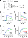
Figure 1.

A, Illustration of the decoder as a linear–nonlinear model neuron. It adds the spikes of all presynaptic neurons in a small time window and multiplies them with a synaptic weight. The result is summed and passed through a nonlinearity, and a threshold is applied. This indicates which of two gratings was presented. B, Time course of the decoding performance for an example session with 20 neurons recorded at 10 and 100% contrast (green and blue lines, respectively) averaged over Δθ. C, Average time course for all 17 sessions sorted by contrast (low contrast: 1–3%, red; medium contrast: 5–30%, green; high contrast: 50–100%, blue) averaged over Δθ. D, Neurometric functions for the example session in B with decoding performance as a function of Δθ. The color code is as in B. E, Average neurometric functions for all 17 sessions sorted by contrast. The color code is as in D.

Figure 2.

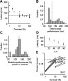
A, Latency as a function of contrast. There are 34 data points in total, 2 for each of the 17 sessions. The dashed line indicates the median latency. B, Distribution of the time to peak performance. The dashed line indicates the median time to peak performance. C, Distribution of the relative performance of the transient period (80–130 ms) versus the sustained period (300–400 ms). The dashed line indicates the median relative performance. D, Mean latency as a function of the difference in orientation, Δθ. E, Peak performance as a function of contrast. The solid lines connect the two data points belonging to the same session. The black dots and lines indicate sessions in which the decoding performance increased with contrast, and the gray dots and lines sessions in which the performance decreased with contrast. The dashed line indicates median peak performance.

Figure 3.

A, Relative peak performance using the integration window size denoted on the x-axis compared with the standard integration window size of 50 ms. The peak performance is computed for each length of the integration window separately and was defined as the performance in the time window that gave the best performance with that integration time. B, Distribution of the relative peak performance of the instantaneous decoder compared with the cumulative decoder for populations (dark) and single neurons (light).

Figure 4.

A, Average firing rate change after stimulus onset compared with baseline (200 to 0 ms before stimulus onset) for all single neurons sorted by contrast (low, medium, and high contrast in red, green, and blue, respectively) averaged over all orientations. Seventy-seven neurons were recorded at low contrast, 180 neurons at medium contrast, and 119 neurons at high contrast. The firing rate profile was smoothed using a Gaussian kernel with SD of ∼30 ms. B, Average Fano factor change after stimulus onset computed and smoothed as in A. C, Average single-unit discriminability d′ change averaged across all combinations of Δθ. D, Average population discriminability d′ change averaged across all combinations of Δθ.

Figure 5.

A, Average absolute weight as a function of time for the three contrast groups (low, medium, and high contrast in red, green, and blue, respectively), renormalized to a maximum of 1 for each contrast separately. B, Average weight as a function of time and the distance of the preferred orientation of a neuron to the decision boundary in the middle of the two orientations that were discriminated. The average is taken across neurons. Weights for medium contrast are shown. The dark color indicates negative weights, and the bright color, positive weights. C, Average weight profile as a function of the distance of the preferred orientation of a neuron to the decision boundary for the three contrast groups (low, medium, and high contrast in red, green, and blue, respectively), renormalized to a maximum of 1 for each contrast separately. D, As in C, but with variability (all contrasts collapsed). Error bars show 1 SD. E, Average weight as a function of the distance between the two gratings that were discriminated and the distance of the preferred orientation of a neuron to the decision boundary. The dark color indicates negative weights, and the bright color, positive weights. F, The normalized weights of the logistic regression decoder (black) compared with the optimal weights assuming that the spike counts of the population follow an independent Poisson distribution (gray) for Δθ = 22.5°.

Figure 6.

A, Relative peak performance of the constant decoder compared with the bin-based one. The dashed line indicates median relative performance. B, Time course of the relative performance of the constant decoder compared with the bin-based one. C, As in B for an additional dataset of sessions in which drifting gratings were shown. Despite the continually changing phase, the relative performance of the constant decoder remains high compared with the bin-based one. D, Comparison of the peak performance using a bin-based or constant decoder for both static (red) and moving (blue) gratings.

Figure 7.

A, Average neurometric functions sorted by the contrast the decoder was tested on (low, medium, and high contrast in red, green, and blue, respectively) showing decoding performance as a function of Δθ, for both a decoder trained and tested on the same contrast (solid) and a decoder trained on data from both contrasts recorded during a single session and tested on one of them (dashed). B, Distribution of the relative peak performance comparing a decoder trained on both contrasts and tested on one of them to one trained and tested on the same contrast. The dashed line indicates median relative performance. C, Average relative peak performance comparing a decoder trained on one contrast and tested on the other (“cross-contrast decoder”) to one trained and tested on the same contrast (“same-contrast decoder”) sorted by the contrast level trained on. Error bars denote SEs of the median. D, As in C, but sorted by the contrast level tested on.

Figure 8.

A, Distribution of the noise correlations between pairs of cells. The dashed line indicates the mean level of correlations. Inset, Average correlation level as a function of contrast level (median ± SE of the median). B, Distribution of the relative peak performance comparing a decoder trained on shuffled data and tested on the real data with one trained and tested on the real data. The dashed line indicates median relative performance. Inset, Average relative performance as a function of contrast level (median ± SE of the median).

Figure 9.

A, Illustration of the model with two subpopulations. The broad subpopulation has a semisaturation contrast of 5% and the narrow subpopulation of 50%. At low contrast (<50%), only the broad subpopulation is activated (top). At high contrasts (>50%), both populations are active (bottom). B, Performance of a decoder discriminating between two gratings 10° apart at low and high contrast using a contrast-specialized decoder (trained and tested on the same contrast; solid), a contrast-independent decoder (trained on both contrasts, tested on one; dashed), and a cross-contrast decoder (trained on one contrast, tested on the other; dotted). The lower contrast was 10% in all cases, while the higher contrast varied between 15 and 100%. C, Relative performance of the contrast-independent and cross-contrast decoders compared with the specialized decoder.

References

1. Albrecht DG, Hamilton DB. Striate cortex of monkey and cat: contrast response function. J Neurophysiol. 1982;48:217–237. - PubMed
1. Averbeck BB, Latham PE, Pouget A. Neural correlations, population coding and computation. Nat Rev Neurosci. 2006;7:358–366. - PubMed
1. Beck JM, Ma WJ, Kiani R, Hanks T, Churchland AK, Roitman J, Shadlen MN, Latham PE, Pouget A. Probabilistic population codes for Bayesian decision making. Neuron. 2008;60:1142–1152. - PMC - PubMed
1. Benucci A, Ringach DL, Carandini M. Coding of stimulus sequences by population responses in visual cortex. Nat Neurosci. 2009;12:1317–1324. - PMC - PubMed
1. Berens P, Ecker AS, Gerwinn S, Tolias AS, Bethge M. Reassessing optimal neural population codes with neurometric functions. Proc Natl Acad Sci U S A. 2011;108:4423–4428. - PMC - PubMed
Publication types
LinkOut - more resources