Perception of climate change

Abstract

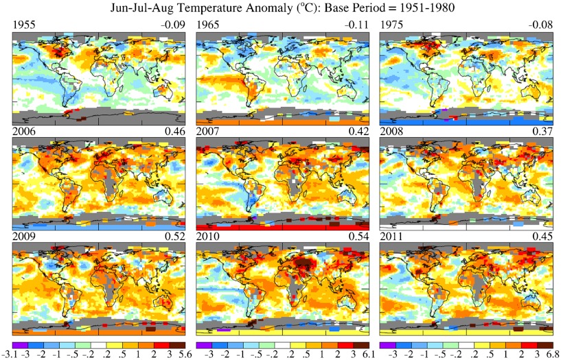
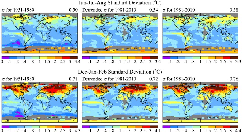
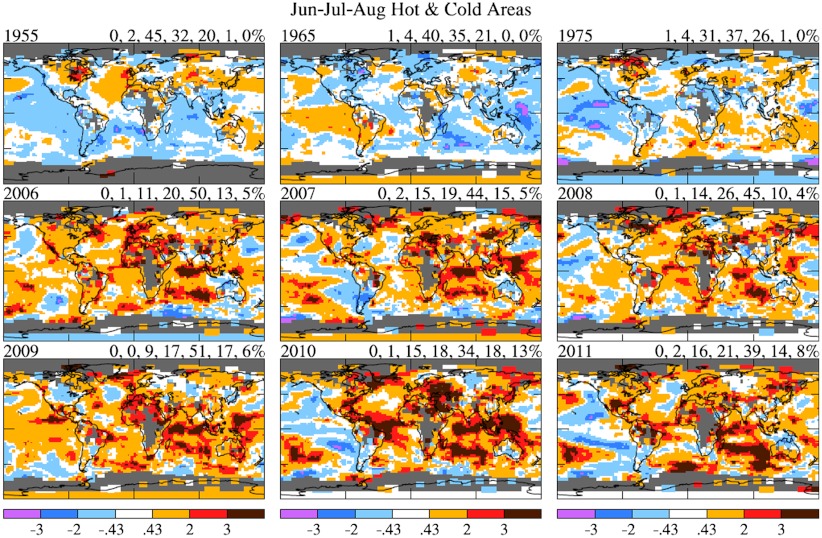
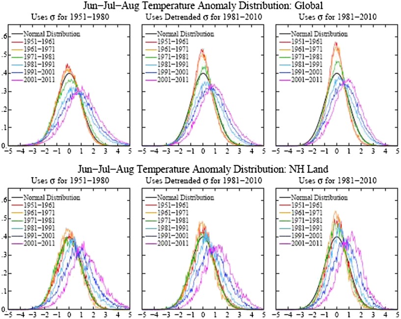
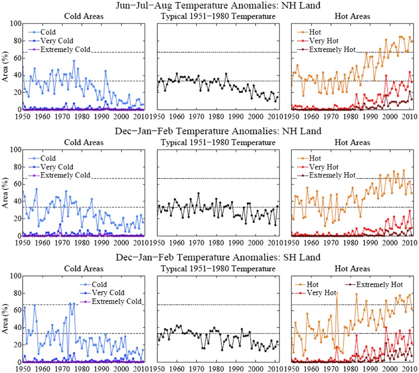
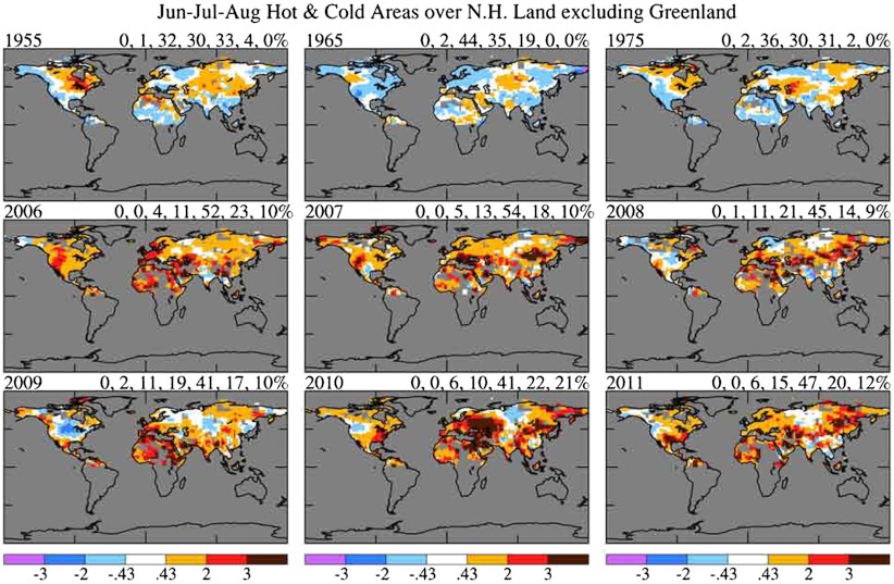
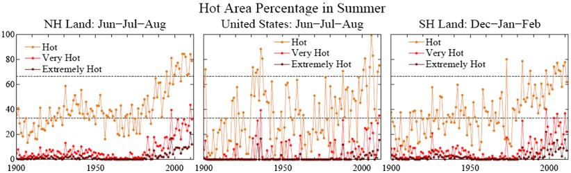
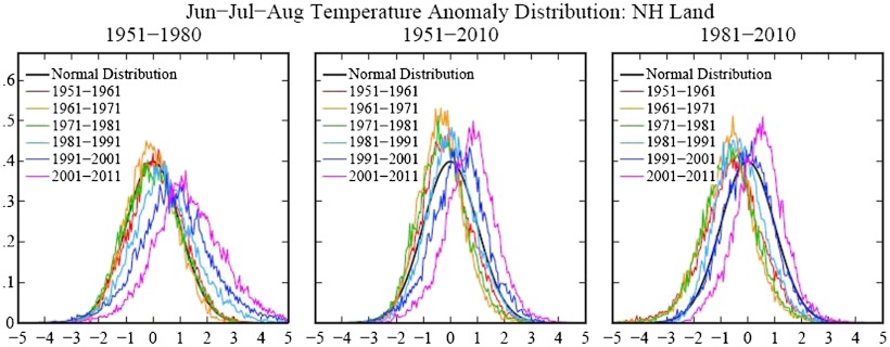
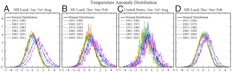
"Climate dice," describing the chance of unusually warm or cool seasons, have become more and more "loaded" in the past 30 y, coincident with rapid global warming. The distribution of seasonal mean temperature anomalies has shifted toward higher temperatures and the range of anomalies has increased. An important change is the emergence of a category of summertime extremely hot outliers, more than three standard deviations (3σ) warmer than the climatology of the 1951-1980 base period. This hot extreme, which covered much less than 1% of Earth's surface during the base period, now typically covers about 10% of the land area. It follows that we can state, with a high degree of confidence, that extreme anomalies such as those in Texas and Oklahoma in 2011 and Moscow in 2010 were a consequence of global warming because their likelihood in the absence of global warming was exceedingly small. We discuss practical implications of this substantial, growing, climate change.

Fig. 1.

June–July–August surface temperature anomalies in 1955, 1965, 1975, and the past 6 y relative to the 1951–1980 mean. Number on Upper Right is the global mean (average over all area with data).

Fig. 2.

Standard deviation of local June–July–August (Upper) and December–January–February (Lower) mean surface temperature for 30-y periods 1951–1980 (Left) and 1981–2010. In the Center maps the local 30-y (1981–2010) temperature trend was removed before calculating the standard deviation.

Fig. 3.

June–July–August surface temperature anomalies in 1955, 1965, 1975, and in 2006–2011 relative to 1951–1980 mean temperature in units of the local detrended 1981–2010 standard deviation of temperature. Numbers above each map are percent of the area with data covered by each category in the color bar.

Fig. 4.

Frequency of occurrence (y axis) of local temperature anomalies (relative to 1951–1980 mean) divided by local standard deviation (x axis) obtained by counting gridboxes with anomalies in each 0.05 interval. Area under each curve is unity.

Fig. 5.

Area covered by temperature anomalies in the categories defined as hot ( > 0.43σ), very hot (> 2σ), and extremely hot (> 3σ), with analogous divisions for cold anomalies. Anomalies are relative to 1951–1980 base period, with σ also from 1951–1980 data. Lowest row is Southern Hemisphere summer.

Fig. 6.

June–July–August surface temperature anomalies over Northern Hemisphere land in 1955, 1965, 1975, and 2006–2011 relative to 1951–1980 base period in units of the local 1951–1980 standard deviation. Numbers above each map are percent of surface area covered by each category in the color bar.

Fig. 7.

Percent area covered by temperature anomalies in categories defined as hot (> 0.43σ), very hot (> 2σ), and extremely hot (> 3σ). Anomalies are relative to 1951–1980 base period; σ is from 1951–1980 data.

Fig. 8.

June–July–August and December–January–February temperature anomalies (°C) relative to 1951–1980 base period for areas shown on the right. Number above each map is the colored region’s percent of global area.

Fig. 9.

Frequency of occurrence (y axis) of local temperature anomalies divided by local standard deviation (x axis) obtained by counting gridboxes with anomalies in each 0.05 standard deviation interval. Area under each curve is unity. Standard deviations are for the indicated base periods.

Fig. P1.

Frequency of occurrence of local temperature anomalies (relative to 1951–1980 mean) divided by local standard deviation obtained by counting gridboxes with anomalies in each 0.05 interval of the standard deviation (x axis). Area under each curve is unity.

References

-
- Rabe BG, Borick CP. Issues in Governance Studies. Washington, DC: Brookings Institution; 2012. Fall 2011 national survey of American public opinion on climate change.
- Hansen J, et al. Target atmospheric CO2: Where should humanity aim? Open Atmos Sci J. 2008;2:217–231.
- Hansen J, et al. Global climate changes as forecast by Goddard Institute for Space Studies 3-dimensional model. J Geophys Res Atmos. 1988;93:9341–9364.
- Solomon S, et al., editors. Intergovernmental Panel on Climate Change (IPCC) Climate Change 2007: The Physical Science Basis. New York, NY: Cambridge press; 2007.
- Hansen J, Ruedy R, Sato M, Lo K. Global surface temperature change. Rev Geophys. 2010;48:RG4004.
Publication types
MeSH terms
LinkOut - more resources
Full Text Sources
Other Literature Sources
Medical
Molecular Biology Databases
Miscellaneous