

A neural network model of ventriloquism effect and aftereffect
- PMID: 22880007
- PMCID: PMC3411784
- DOI: 10.1371/journal.pone.0042503
A neural network model of ventriloquism effect and aftereffect
Abstract
Presenting simultaneous but spatially discrepant visual and auditory stimuli induces a perceptual translocation of the sound towards the visual input, the ventriloquism effect. General explanation is that vision tends to dominate over audition because of its higher spatial reliability. The underlying neural mechanisms remain unclear. We address this question via a biologically inspired neural network. The model contains two layers of unimodal visual and auditory neurons, with visual neurons having higher spatial resolution than auditory ones. Neurons within each layer communicate via lateral intra-layer synapses; neurons across layers are connected via inter-layer connections. The network accounts for the ventriloquism effect, ascribing it to a positive feedback between the visual and auditory neurons, triggered by residual auditory activity at the position of the visual stimulus. Main results are: i) the less localized stimulus is strongly biased toward the most localized stimulus and not vice versa; ii) amount of the ventriloquism effect changes with visual-auditory spatial disparity; iii) ventriloquism is a robust behavior of the network with respect to parameter value changes. Moreover, the model implements Hebbian rules for potentiation and depression of lateral synapses, to explain ventriloquism aftereffect (that is, the enduring sound shift after exposure to spatially disparate audio-visual stimuli). By adaptively changing the weights of lateral synapses during cross-modal stimulation, the model produces post-adaptive shifts of auditory localization that agree with in-vivo observations. The model demonstrates that two unimodal layers reciprocally interconnected may explain ventriloquism effect and aftereffect, even without the presence of any convergent multimodal area. The proposed study may provide advancement in understanding neural architecture and mechanisms at the basis of visual-auditory integration in the spatial realm.
Conflict of interest statement
Figures
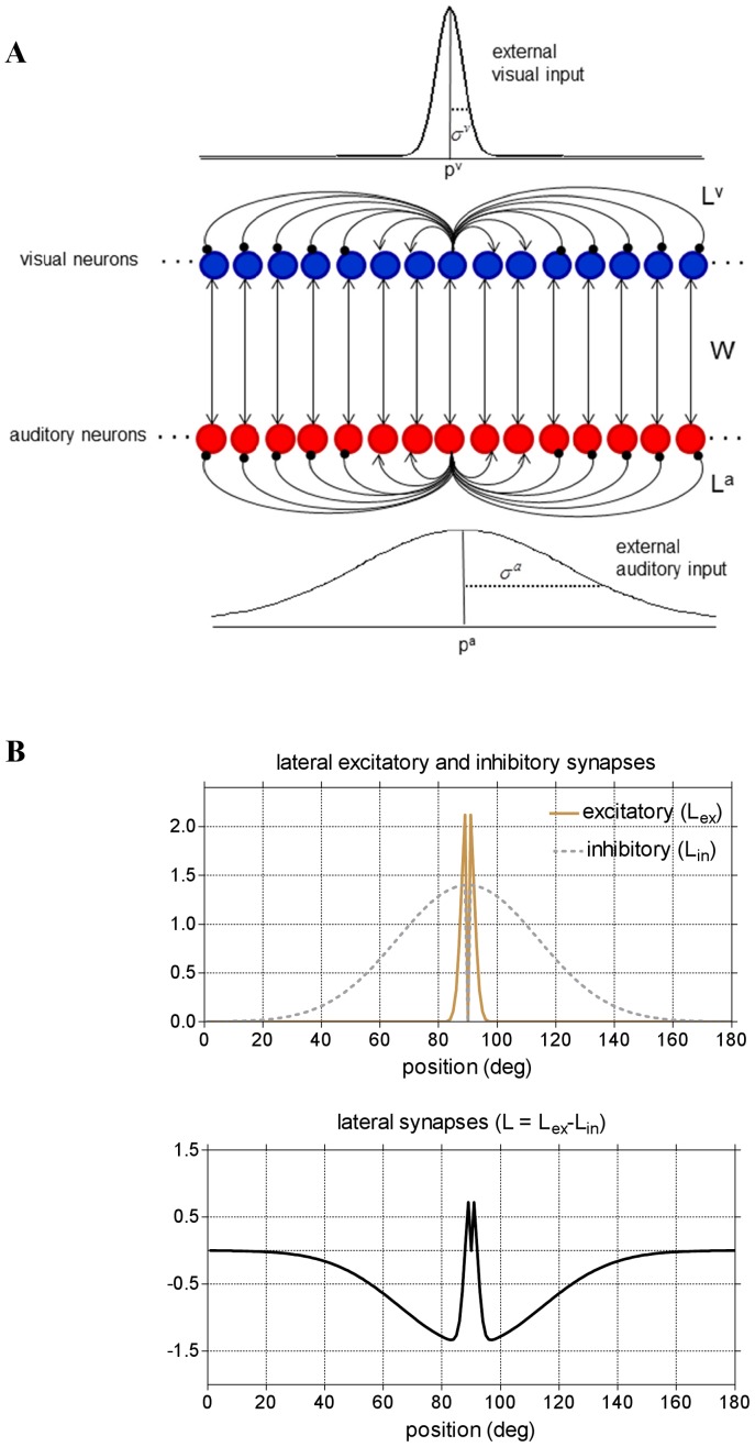
 . The fundamental assumption is σa>σv. Neurons between layers are connected via excitatory inter-area synapses (strength W). Neurons within each layers are connected via lateral (excitatory and inhibitory) synapses. For simplicity, only lateral synapses emerging from one neuron are displayed. In basal conditions, each neuron receives and sends symmetrical lateral synapses. (B) Pattern of the lateral synapses targeting (or emerging from) an exemplary neuron in either layer, in pre-training condition. Lateral excitatory (Lex) and inhibitory (Lin) synapses have a Gaussian pattern with excitation stronger but narrower than inhibition. Auto-excitation and auto-inhibition are excluded. Net lateral synapses (L) are obtained as the difference between excitatory and inhibitory synapses and assume a “Mexican hat” disposition.
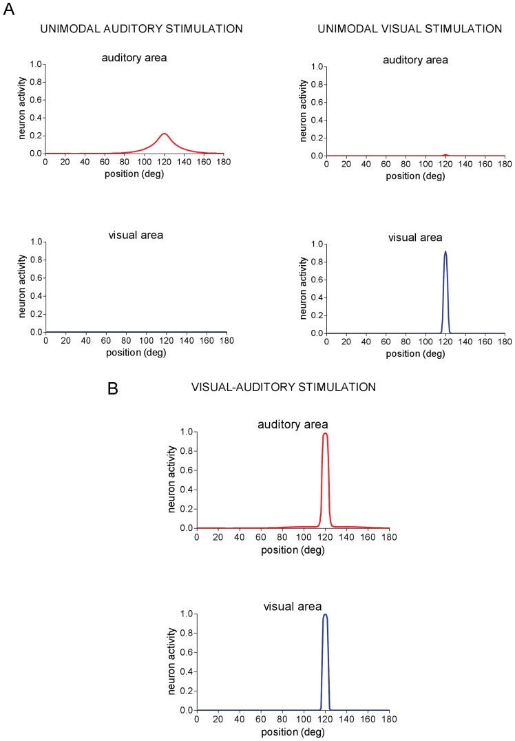
 = 15 applied at position pa = 120°. No activity is elicited in the visual area. Right panels - Neuron activity in the auditory and visual areas in response to a visual stimulus of amplitude
  = 15 applied at position pv = 120°. No significant activity is elicited in the auditory area. (B) An auditory stimulus and a visual stimulus are simultaneously applied at the same spatial position (pa = pv = 120°) and maintained constant throughout the simulation. Network response is shown in steady-state condition. Auditory and visual stimuli have the same strength (
 =
=  = 15). Strong reinforcement and narrowing of auditory activation occurs (compare with Fig. 2A, left panels).
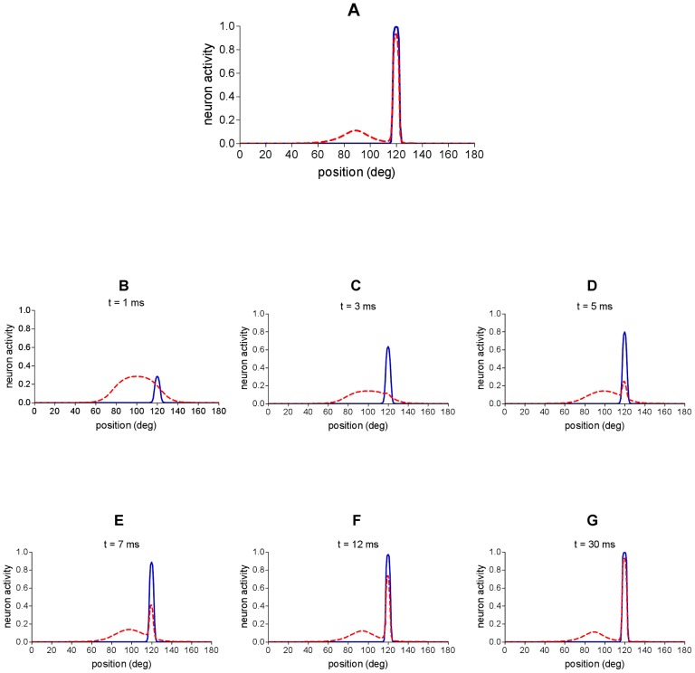
 =
=  = 15). Dashed red line represents activity in the auditory area; continuous blue line represents activity in the visual area. (A) Network activity in the final steady-state reached by the network. (B–G) Different snapshots of network activity during the simulation. First snapshot (B) depicts network activity immediately after the stimuli presentation; last snapshot (G) corresponds to the final state reached by the network.
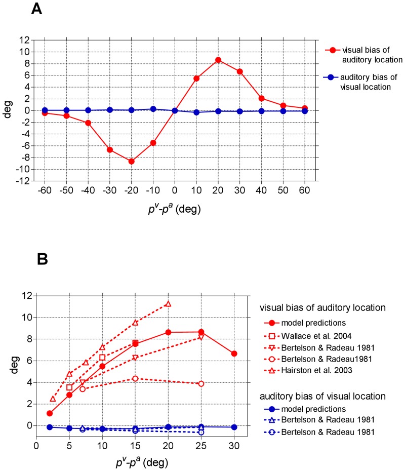
 =
=  = 15). (B) Comparison between model predictions and in-vivo data. Biases predicted by the model (same results as (A)) are zoomed between 0° and 30° of visual-auditory angular separation for comparison with in-vivo data.
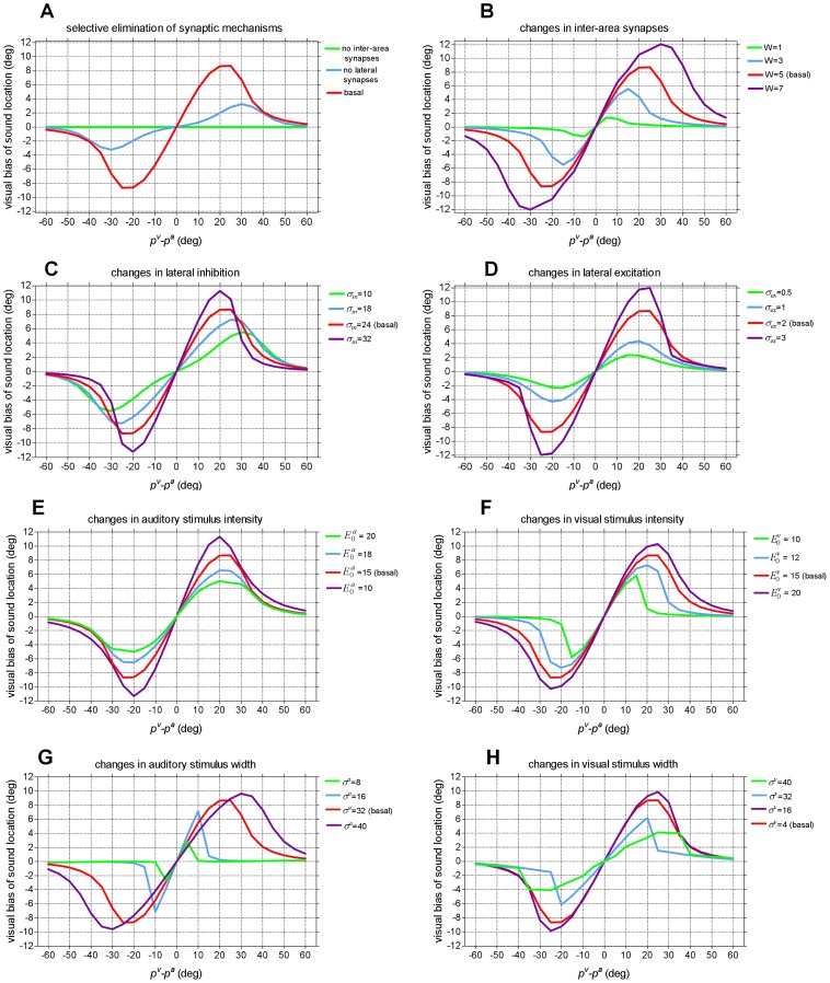
 ). (F) Changes in the strength of the visual stimulus (
 ). (G) Changes in the width of the auditory stimulus (σa). (H) Changes in the width of the visual stimulus (σv).
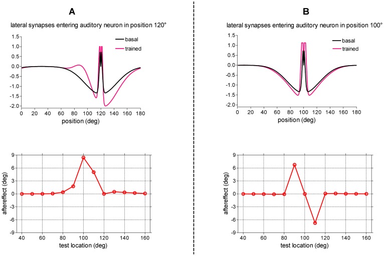
 = 15, and was applied at different positions. For each position of the test stimulus, the shift in sound localization (perceived stimulus location minus original stimulus location) was computed in steady-state condition (after the transient response was exhausted) and reported as a function of the actual location of the test auditory stimulus (aftereffect). (B) Case 1.b: training with spatially coincident stimuli in fixed position (pv = 100°, pa = 100°). Upper panel: Lateral synapses entering the auditory neuron in position 100° before and after training. Lower panel: Behavior of the trained network in response to auditory unimodal stimulation. The same unimodal auditory test as panel A was performed to compute the aftereffect.
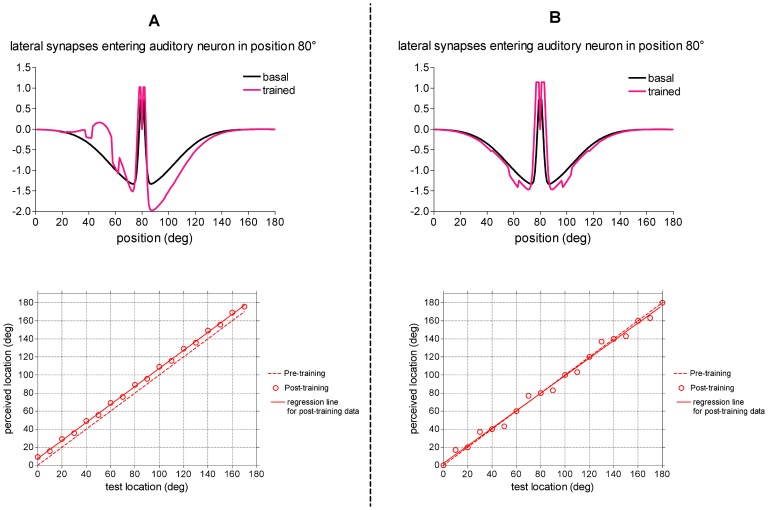
 = 15, and was applied at different positions. The perceived sound location, computed in steady-state condition, was reported as a function of the original location of the test stimulus (values represented by circles). For comparison, the behavior of the untrained network was shown too (dashed line). The regression line for the post-training data (continuous line) has slope 1 and offset ∼7.5° (r2 = 0.9990, p<0.0001). (B) Case 2.b: training with spatially coincident stimuli in variable position. The auditory stimulus could be located in one among nine positions (from 20° to 180° with 20° step), and the simultaneous visual stimulus was located in the same spatial position (pv = pa). The overall training procedure was the same as panel A (but with spatially coincident stimuli). Upper panel: Lateral synapses entering an exemplary auditory neuron (neuron in position 80°, one of the trained position) are shown before and after the training. Lower panel: Behavior of the trained network in response to auditory unimodal stimulation. The same auditory unimodal test as in panel A was performed. In this case, the regression line for the post-training data is almost indistinguishable from the pre-training line.
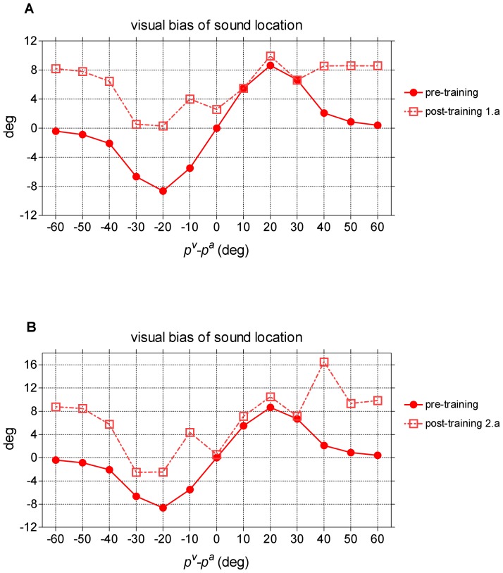
Similar articles
-
A neural network model can explain ventriloquism aftereffect and its generalization across sound frequencies.Biomed Res Int. 2013;2013:475427. doi: 10.1155/2013/475427. Epub 2013 Oct 21. Biomed Res Int. 2013. PMID: 24228250 Free PMC article.
-
Accumulation and decay of visual capture and the ventriloquism aftereffect caused by brief audio-visual disparities.Exp Brain Res. 2017 Feb;235(2):585-595. doi: 10.1007/s00221-016-4820-4. Epub 2016 Nov 11. Exp Brain Res. 2017. PMID: 27837258 Free PMC article.
-
A neurocomputational analysis of the sound-induced flash illusion.Neuroimage. 2014 May 15;92:248-66. doi: 10.1016/j.neuroimage.2014.02.001. Epub 2014 Feb 9. Neuroimage. 2014. PMID: 24518261
-
[Ventriloquism and audio-visual integration of voice and face].Brain Nerve. 2012 Jul;64(7):771-7. Brain Nerve. 2012. PMID: 22764349 Review. Japanese.
-
Rapidly induced auditory plasticity: the ventriloquism aftereffect.Proc Natl Acad Sci U S A. 1998 Feb 3;95(3):869-75. doi: 10.1073/pnas.95.3.869. Proc Natl Acad Sci U S A. 1998. PMID: 9448253 Free PMC article. Review.
Cited by
-
A Computational Analysis of Neural Mechanisms Underlying the Maturation of Multisensory Speech Integration in Neurotypical Children and Those on the Autism Spectrum.Front Hum Neurosci. 2017 Oct 30;11:518. doi: 10.3389/fnhum.2017.00518. eCollection 2017. Front Hum Neurosci. 2017. PMID: 29163099 Free PMC article.
-
The Ventriloquist Illusion as a Tool to Study Multisensory Processing: An Update.Front Integr Neurosci. 2019 Sep 12;13:51. doi: 10.3389/fnint.2019.00051. eCollection 2019. Front Integr Neurosci. 2019. PMID: 31572136 Free PMC article.
-
A neural network model can explain ventriloquism aftereffect and its generalization across sound frequencies.Biomed Res Int. 2013;2013:475427. doi: 10.1155/2013/475427. Epub 2013 Oct 21. Biomed Res Int. 2013. PMID: 24228250 Free PMC article.
-
Processing of audiovisually congruent and incongruent speech in school-age children with a history of specific language impairment: a behavioral and event-related potentials study.Dev Sci. 2015 Sep;18(5):751-70. doi: 10.1111/desc.12263. Epub 2014 Nov 29. Dev Sci. 2015. PMID: 25440407 Free PMC article.
-
Accumulation and decay of visual capture and the ventriloquism aftereffect caused by brief audio-visual disparities.Exp Brain Res. 2017 Feb;235(2):585-595. doi: 10.1007/s00221-016-4820-4. Epub 2016 Nov 11. Exp Brain Res. 2017. PMID: 27837258 Free PMC article.
References
-
- Stein BE, Meredith MA (1993) The merging of the senses. Cambridge, MA: The MIT Press.
-
- Bertelson P, Radeau M (1981) Cross-modal bias and perceptual fusion with auditory-visual spatial discordance. Percept Psychophys 29: 578–584. - PubMed
-
- Radeau M, Bertelson P (1987) Auditory-Visual Interaction and the Timing of Inputs - Thomas (1941) Revisited. Psychological Research-Psychologische Forschung 49: 17–22. - PubMed
-
- Radeau M, Bertelson P (1977) Adaptation to auditory-visual discordance and ventriloquism in semirealistic situations. Percept Psychophys 22: 137–146.
-
- Welch RB, Warren DH (1980) Immediate perceptual response to intersensory discrepancy. Psychol Bull 88: 638–667. - PubMed
MeSH terms
LinkOut - more resources
Full Text Sources
