Finding low-energy conformations of lattice protein models by quantum annealing

Abstract

Lattice protein folding models are a cornerstone of computational biophysics. Although these models are a coarse grained representation, they provide useful insight into the energy landscape of natural proteins. Finding low-energy threedimensional structures is an intractable problem even in the simplest model, the Hydrophobic-Polar (HP) model. Description of protein-like properties are more accurately described by generalized models, such as the one proposed by Miyazawa and Jernigan (MJ), which explicitly take into account the unique interactions among all 20 amino acids. There is theoretical and experimental evidence of the advantage of solving classical optimization problems using quantum annealing over its classical analogue (simulated annealing). In this report, we present a benchmark implementation of quantum annealing for lattice protein folding problems (six different experiments up to 81 superconducting quantum bits). This first implementation of a biophysical problem paves the way towards studying optimization problems in biophysics and statistical mechanics using quantum devices.

Figure 1. Device architecture and qubit connectivity.

The array of superconducting quantum bits is arranged in 4 × 4 unit cells that consist of 8 quantum bits each. Within a unit cell, each of the 4 qubits in the left-hand partition (LHP) connects to all 4 qubits in the right-hand partition (RHP), and vice versa. A qubit in the LHP (RHP) also connects to the corresponding qubit in the LHP (RHP) of the units cells above and below (to the left and right of) it. (a) Qubits are labeled from 0 to 127 and edges between qubits represent couplers with programmable coupling strengths. Grey qubits indicate the 115 usable qubits, while vacancies indicate qubits under calibration which were not used. The larger experiments (Experiments 1,2, and 4) were performed on this chip, while the three remaining smaller experiments were run on other chips with the same architecture. (b) Embedding and qubit connectivity for Experiment 4, coloring the 81 qubits used in the experiment. Nodes with the same color represent the same logical qubit from the original 19-qubit Ising-like Hamiltonian resulting from the energy function associated with Experiment 4 (see Supplementary material for details). This embedding aims to fulfill the arbitrary connectivity of the Ising expression and allows for the coupling of qubits that are not directly coupled in hardware.

Figure 2. Lattice folding mapping for quantum annealing.

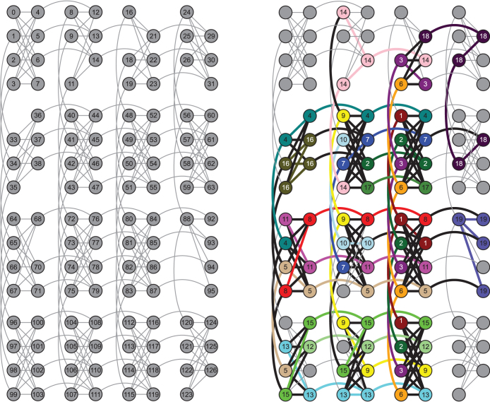
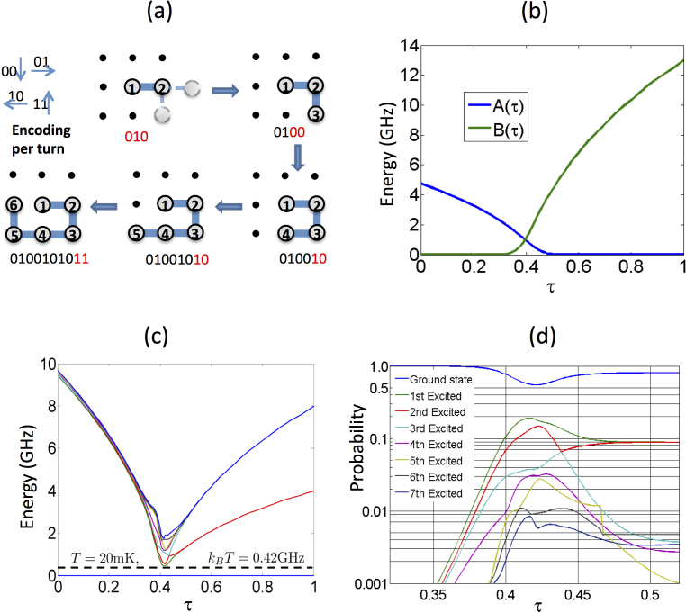
(a) Step-by-step construction of the binary representation of lattice protein. Two qubits per bond are needed and the bond directions are denoted as “00” (downwards), “01” (rightwards), “10” (leftwards), and “11” (upwards). The example shows one of the possible folds of an arbitrary six-amino-acid sequence. Any possible N-amino-acid fold can be represented by a string of variables with . (b)Time-dependence of the A(τ) and B(τ) functions, where τ = t/t_run with t_run = 148 µs, (c) time-dependent spectrum obtained through numerical diagonalization, and (d) Bloch-Redfield simulations showing the time-dependent population in the first eight instantaneous eigenstates of the experimentally implemented 8-qubit Hamiltonian (Eq. 3) with H_p from Eq. S18 in the Supplementary material. In panel (c), for each instantaneous eigenenergy curve we have subtracted the energy of the ground state, effectively plotting the gap of the seven-lowest-excited states with respect to the ground state (represented by the baseline at zero-energy). As a reference, we show the energy with the device temperature, which is comparable to the minimum gap between the ground and first excited state. In panel (d), populations are ordered in energy from top (ground state) to bottom. Although τ = t/t_run runs from 0 to 1, we show the region where most of the population changes occur. As expected, this is in the proximity of the minimum gap between the ground and first excited state around τ ~ 0.4 [see panel(c)].

Figure 3. Experimental realizations.

(a) Representation of the six-amino-acid sequence, Proline-Serine-Valine-Lysine-Methionine-Alanine with its respective one-letter sequence notation, PSVKMA. We use the pairwise nearest-neighbor Miyazawa-Jernigan interaction energies reported in Table 3 of Ref. . (b) Divide and conquer approach showing three different schemes which independently solve the six-amino-acid sequence PSVKMA on a two-dimensional lattice. We solved the problem under Scheme2 and 3 (Experiments 1 through 4). (c) Energy landscape for the valid conformations of the PSVKMA sequence. Results of the experimentally-measured probability outcomes are given as color-coded percentages according to each of the experimental realizations described in panel (b). Percentages for states with energy greater than zero are 32.70%, 59.88%, 8.00%, and 95.97% for Experiments 1 through 4, respectively.

Figure 4. Embedding problem instances into hardware.

Graph representations of (a) the four-qubit unembedded energy function (Eq. 6) and (b) the five-qubit expression (Eq. 7) as was embedded into the quantum hardware. In graphs (a) and (b), each node denotes a qubit and the color and extent of its glow denotes the sign and strength of its corresponding longitudinal field, h_i. The edges represent the interaction couplings, J_ij, where color indicates sign and thickness indicates magnitude. Since we want the two qubits representing q₄ (q₄ and q_4′) to end up with the same value, we apply the maximum ferromagnetic coupling (J = −1) between them, which adds a penalty whenever this equality is violated. These maximum couplings are indicated in the figure by heavy lines. For the case of Experiment 3, the reconstruction of the binary bit stings representing the folds in Fig. 3, from the five-qubit experimental measurements can be recovered by q_exp3 = 010010q₁0q₂q₃|q₄q_4′, with q_i = 0 (q_i = 1) whenever s_i = 1 (s_i = −1).

References

-
- Šali A., Shakhnovich E. & Karplus M. How does a protein fold? Nature 369, 248–251 (1994). - PubMed
- Pande V. S. Simple theory of protein folding kinetics. Phys. Rev. Lett. 105, 198101 (2010). - PubMed
- Mirny L. & Shakhnovich E. Protein folding theory: from lattice to all-atom models. Annu. Rev. Biophys. Bio. 30, 361–396 (2001). - PubMed
- Pande V. S., Grosberg A. Y. & Tanaka T. Heteropolymer freezing and design: Towards physical models of protein folding. Rev. Mod. Phys. 72, 259 (2000).
Publication types
MeSH terms
Substances
LinkOut - more resources
Full Text Sources
Other Literature Sources
Research Materials
Miscellaneous