Spectrotemporal contrast kernels for neurons in primary auditory cortex

Abstract

Auditory neurons are often described in terms of their spectrotemporal receptive fields (STRFs). These map the relationship between features of the sound spectrogram and firing rates of neurons. Recently, we showed that neurons in the primary fields of the ferret auditory cortex are also subject to gain control: when sounds undergo smaller fluctuations in their level over time, the neurons become more sensitive to small-level changes (Rabinowitz et al., 2011). Just as STRFs measure the spectrotemporal features of a sound that lead to changes in the firing rates of neurons, in this study, we sought to estimate the spectrotemporal regions in which sound statistics lead to changes in the gain of neurons. We designed a set of stimuli with complex contrast profiles to characterize these regions. This allowed us to estimate the STRFs of cortical neurons alongside a set of spectrotemporal contrast kernels. We find that these two sets of integration windows match up: the extent to which a stimulus feature causes the firing rate of a neuron to change is strongly correlated with the extent to which the contrast of that feature modulates the gain of the neuron. Adding contrast kernels to STRF models also yields considerable improvements in the ability to capture and predict how auditory cortical neurons respond to statistically complex sounds.

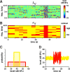
Figure 1.

Stimuli used to estimate contrast kernels and their statistics. A, Schematic of an RC-DRC stimulus. The stimulus comprises a sequence of chords, which change every 25 ms. The elements of the chords are pure tones, whose levels are drawn from one of the distributions shown in C. The color grid shows the sound level (L_tf) of a particular tone frequency at a particular time. B, The 38 s DRC stimulus shown in A comprises 12 segments in which the contrast in different frequency bins, σ_tf, is either high (red) or low (yellow). C, Tone level distributions for low (yellow) and high (red) contrast segments. D, Level as a function of time for the 2.4 kHz tone over a 9 s period, i.e., a cross-section of A. This shows the transition from a segment in which the level distribution of this tone was low contrast (yellow), to a segment in which it was high contrast (red), to a third segment in which it was low contrast again (yellow).

Figure 2.

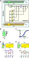
Schematic of the contrast kernel model. A, The relationship between stimulus and neuronal response. The sound input is represented by its spectrogram, L_tf (top), and by its contrast profile, σ_tf (bottom). As in a standard LN model, the neural response is determined by convolving the spectrogram with a linear spectrotemporal kernel (k_fh) and passing the output of this operation (x_t) through a static output nonlinearity (here, a 4-parameter sigmoid, denoted by the blue curve) to produce the predicted spike rate (ŷ_t). The model developed here extends this by allowing each of the four parameters of the output nonlinearity (a–d, as shown in C) to change over time, depending on the statistics of recent stimulation. The evolution of each parameter θ ϵ {a, b, c, d} over time is determined by convolving the contrast profile of the sound, σ_tf, with a linear contrast kernel, κ_fh^(θ). The effects of this on the shape of the output nonlinearity are illustrated in D and E. B, All STRFs and contrast kernels are assumed to be separable in frequency and time, such that k_fh = k_f ⊗ k_h, and κ_fh^(θ) = κ_f^(θ) ⊗ κ_h^(θ). This allows contrast kernels to be fitted in two stages: (1) the spectral component (SCKs) in Figures 3–6 and (2) the temporal component (TCKs) in Figure 7. C, The parameters of a sigmoidal static nonlinearity: a, the minimum firing rate; b, the output dynamic range; c, the stimulus inflection point; d, the (inverse) gain. D, An illustration of the effect of a contrast kernel for the nonlinearity parameter a, which sets the minimum firing rate of the output nonlinearity. Top left, A contrast kernel κ_fh^(a) is shown. Top right, The contrast profile of an example stimulus. Middle right, As a result of changing contrast, the parameter a changes with time. Bottom right, The effective shape of the output nonlinearities at different times attributable to the changing value of a. These shifts would be combined with the contrast-dependent changes to the other nonlinearity parameters, b, c, and d, such as shown in E. E, Effect of a contrast kernel for the nonlinearity parameter d, which sets the (inverse) gain of the output nonlinearity. This neuron decreases its gain when there is high contrast anywhere within a relatively broad region demarcated by κ_fh^(d).

Figure 3.

Including SCKs in models of neural responses improves their predictive power over the LN model; this is further improved by simplifying the model. A, Model predictive power, as measured by Sahani and Linden (2003). Model names are defined in Materials and Methods. For each model, scatter plots show the cross-validated prediction scores across all 77 units. These are calculated as the percentage of the signal power (%SPE) of the unit captured by the model on the prediction dataset and shown as a function of the normalized noise power in the responses of the unit. Gray line shows the extrapolation of prediction scores to an idealized zero-noise unit, producing a lower bound on the overall predictive power of the model over the population of auditory cortical units. The upper bound on predictive power has been omitted for clarity. B, Summary of predictive powers for the models in A. Solid bars show the lower bound (as plotted in A) from cross-validation; error bars show the upper bound from the training dataset. Although adding a full set of contrast kernels (a/b/c/d) leads to a modest improvement in prediction scores over the LN model, the large number of parameters in the full model leads to overfitting. Rendering a and b contrast independent reduces overfitting and improves prediction scores (the c/d model). The best-performing model is the cd model, with a shared contrast kernel between c and d. C, Comparison between prediction scores for the LN model and for the STRF model, on a unit-by-unit basis. D, Comparison between the LN model and cd model on a unit-by-unit basis.

Figure 4.

Gain model: contrast-dependent gain changes across the population of A1/AAF units. A, The majority of units decreased their gain as contrast was increased, as expected. This is measured here by the radio G_d = d_high/d_low. B, The larger the contrast-dependent gain of a unit changes, the greater the improvement in model predictive power over the standard LN model. The (nonparametric) Spearman's correlation coefficient between G_d and model improvement was 0.40 (p < 0.001).

Figure 5.

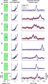
Gain SCKs, for eight example units. These are fits of the cd model, with contrast-independent a and b, and a shared, real-valued SCK, κ_f^(cd), for c and d. Left, STRF for each unit. Middle, Static output nonlinearities for each unit, when estimated under the all-high-contrast condition (magenta) and the all-low-contrast condition (cyan), showing the gain change between the two conditions. Right, SCK for each unit. The black line shows the MAP estimate for κ_f^(cd); the red filled region, bounded by the gray lines, shows a 95% credible interval for the posterior distribution over these coefficients. The red shading increases in darkness with probability. The blue line and blue diamonds show the frequency component of the linear, separable STRF, k_f. Both k_f and κ_f^(cd) have been normalized by the respective SDs to facilitate visual comparison. A–D exemplify how k_f and κ_f^(cd) align in BF and bandwidth. E–G (but not H) show examples in which κ_f^(cd) covers the inhibitory sidebands of the receptive field.

Figure 6.

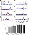
Approximations to the cd model. A–H, Gain SCKs when coefficients were constrained to be positive. This shows the same eight units as shown in Figure 5. Again, the frequency component of the STRF, k_f (blue), approximately matches the gain SCK, κ_f^(cd) (black line and red area). I, Model predictive power for the cd model with constrained coefficients; as in Figure 3B, solid bars show prediction scores, and error bars show training scores. When the contrast kernel coefficients are unconstrained (κ ϵ ℜ; right), the model performance is better than the linear (STRF) and LN models (left). Restricting the coefficients of the SCK to be positive (κ > 0) reduces overfitting and improves prediction scores. Excellent approximations are provided by fixing the SCKs as either the absolute value of the STRF frequency kernel (κ = |k|) or the rectified value (κ = |k|⁺). Models that do not perform as well include fixing the contrast kernel as the STRF frequency kernel (κ = k), fixing it as the magnitude of the Hilbert transform of the STRF frequency kernel (κ = |H(k)|), or assuming that it is constant with respect to frequency (κ = 1). These still outperform the simple LN model. Dashed lines are shown at the model performance values for the LN model and the constrained-positive cd model.

Figure 7.

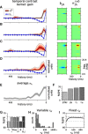
TCKs. A–D, Left panels show the TCKs for four example units. As in Figures 5 and 6, red area shows the gain TCK, κ_h^(cd), whereas blue line and diamonds show the temporal component of the STRF, k_h. Right panels compare the STRF, k_fh, with the full STCKs, κ_fh^(cd), as per Figure 2. E, Mean of the contrast time kernels from the 77 cortical units, ¯κ_h^(cd). This shows the approximately exponential shape of the time kernels. The mean contrast kernel had a fitted time constant of 86 ms. F, Model predictive power. Including a history component to the contrast kernels (κ_fh) improves the performance of the model compared with the assumption that only the current contrast matters (κ_f). Prediction scores for the simple STRF model and the LN model are shown for comparison. Note that this is fitted over a different dataset from that used in Figures 3–6, so the values of %SPE in this figure do not match those presented previously. G, Model predictive powers for a range of TCK models. In order, from left to right, these models are the following: (κ_f), no history dependence, i.e., κ_h = δ_h0; (τ), exponential model with time constant τ_H fitted (see H); (85 ms), exponential model with τ_H fixed at 85 ms (see I); (>0), κ_h constrained to be positive; (ℜ), κ_h allowed to take on any real value; (|k_h|), κ_h approximated as the absolute value of the STRF time kernel. Dashed horizontal lines show the model predictive power for the κ_f and the >0 models. Note that allowing the coefficients of the TCK to be real-valued (the ℜ model) led to considerable overfitting; the >0 model is thus the STCK model considered in Materials and Methods. H, Fits of the time constant τ_H for the exponential model for all 77 units. The median time constant was 117 ms. I, Model predictive power for the exponential model when τ_H was fixed rather than fitted. Abscissa denotes the fixed value of τ_H, ordinate as in G. The horizontal dashed lines are as in G. The most predictive model had τ_H = 85 ms. Thus, three different measures of the time course of gain changes (in E, H, and I) give approximately consistent answers.

Figure 8.

Summary of results. We find that the gain changes undergone by cortical neurons in response to complex patterns of stimulus contrast can be captured by this simplified contrast kernel model. The neural response is determined by convolving the spectrogram with a linear spectrotemporal kernel (k_fh) and passing the output of this operation (x_t) through a static output nonlinearity to produce the predicted spike rate (ŷ_t). The minimum and maximum firing rate of the output nonlinearity are fixed, but the stimulus inflection point (c) and the (inverse) gain (d) change over time, depending on the statistics of recent stimulation. The evolution of c and d over time is determined by convolving the contrast profile of the sound, σ_tf, with a single contrast kernel, κ_fh^(cd), as in Equation 11. Finally, the contrast kernel can be approximated as κ_fh^(cd) ≈ |k_fh|. This model captures 20–25% of the residual variance not explained by the LN model by adding only an additional two parameters.

References

1. Abolafia JM, Vergara R, Arnold MM, Reig R, Sanchez-Vives MV. Cortical auditory adaptation in the awake rat and the role of potassium currents. Cereb Cortex. 2011;21:977–990. - PubMed
1. Aertsen AM, Johannesma PI. The spectro-temporal receptive field. Biol Cybern. 1981;42:133–143. - PubMed
1. Aertsen AM, Johannesma PI, Hermes DJ. Spectro-temporal receptive fields of auditory neurons in the grassfrog. II. Analysis of the stimulus-event relation for tonal stimuli. Biol Cybern. 1980;38:235–248. - PubMed
1. Ahrens MB, Linden JF, Sahani M. Nonlinearities and contextual influences in auditory cortical responses modeled with multilinear spectrotemporal methods. J Neurosci. 2008a;28:1929–1942. - PMC - PubMed
1. Ahrens MB, Paninski L, Sahani M. Inferring input nonlinearities in neural encoding models. Network. 2008b;19:35–67. - PubMed
Publication types
LinkOut - more resources