. 2012 Aug 15;32(33):11396-413.
doi: 10.1523/JNEUROSCI.0429-12.2012.

Response properties of local field potentials and neighboring single neurons in awake primary visual cortex

Affiliations

Response properties of local field potentials and neighboring single neurons in awake primary visual cortex

Reza Lashgari et al. J Neurosci. .

Abstract

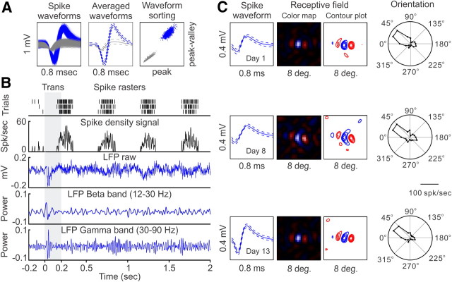
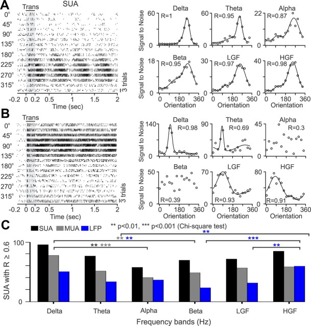
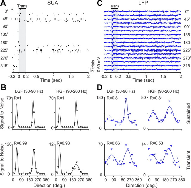
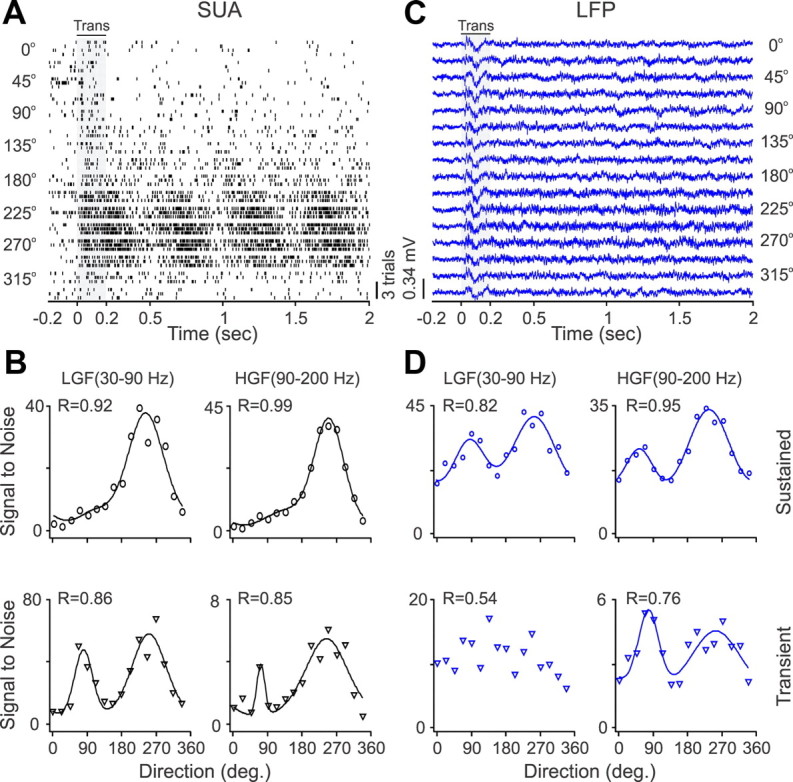
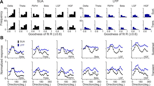
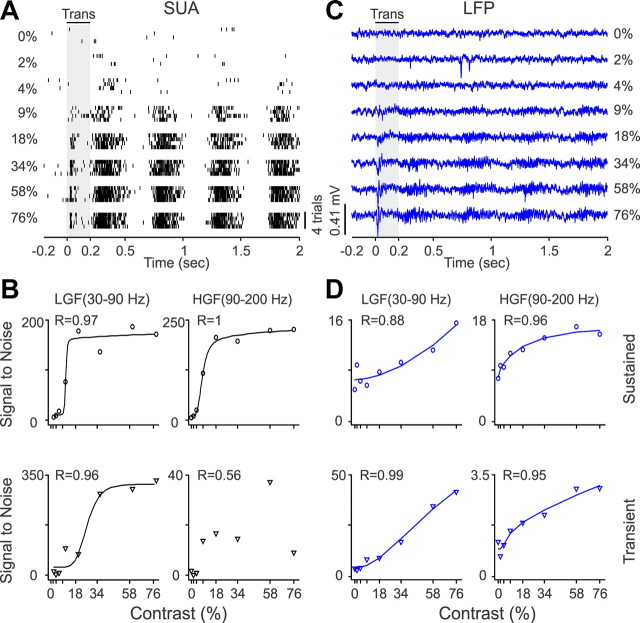
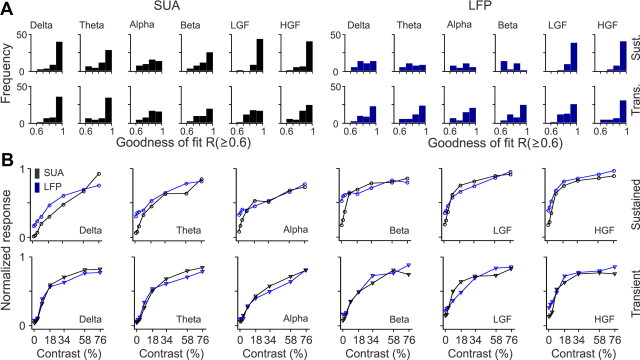
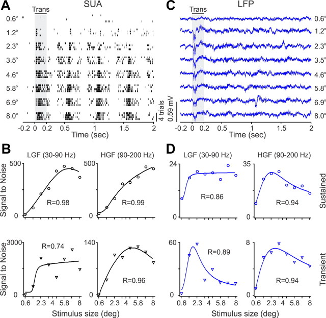
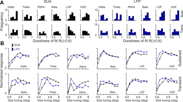
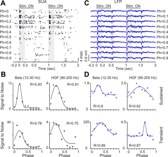
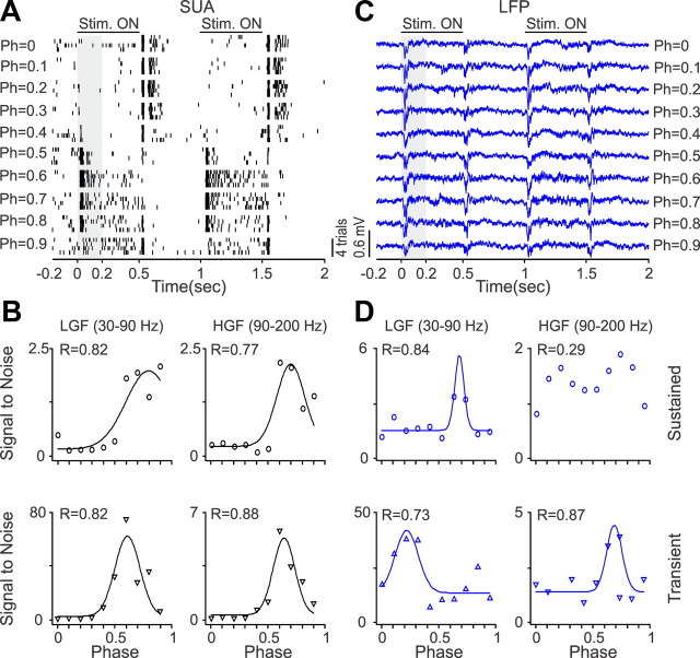
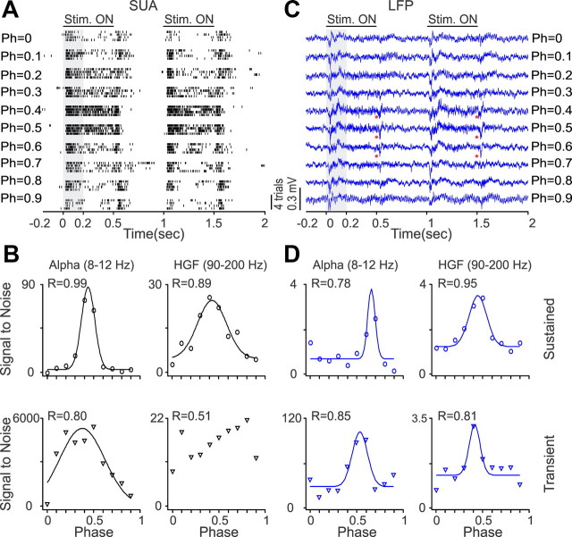
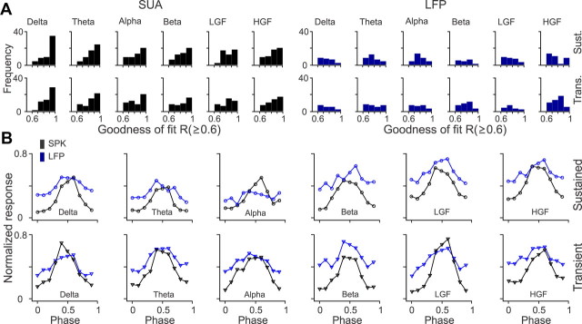
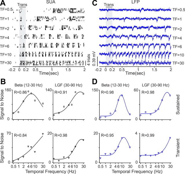
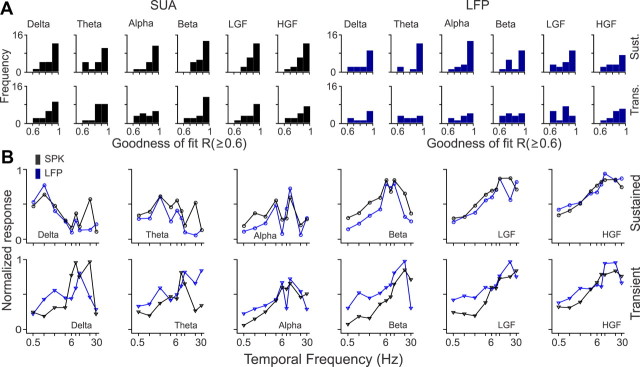
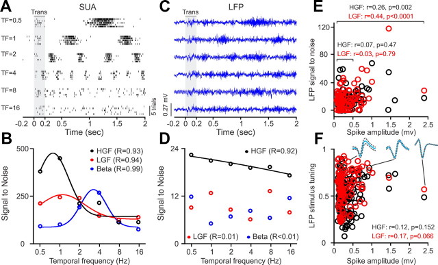
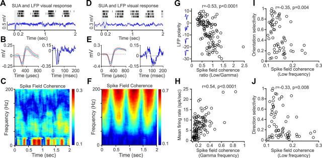
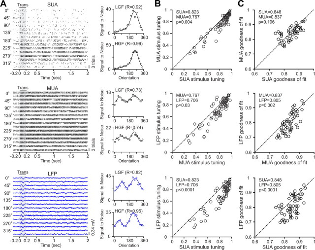
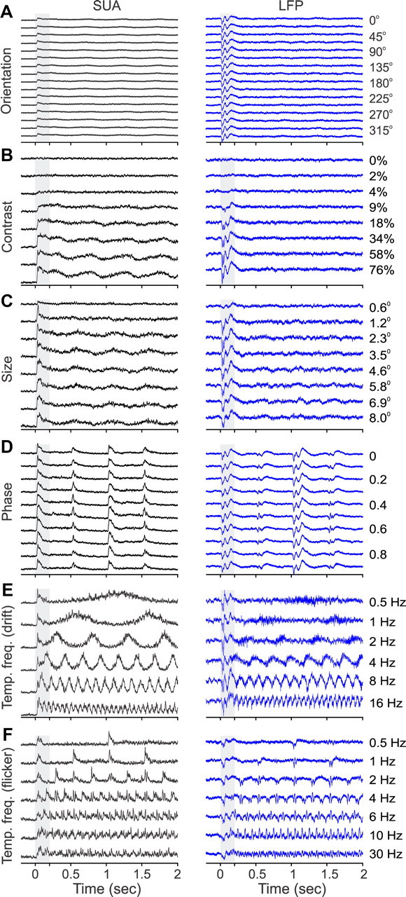
Recordings from local field potentials (LFPs) are becoming increasingly common in research and clinical applications, but we still have a poor understanding of how LFP stimulus selectivity originates from the combined activity of single neurons. Here, we systematically compared the stimulus selectivity of LFP and neighboring single-unit activity (SUA) recorded in area primary visual cortex (V1) of awake primates. We demonstrate that LFP and SUA have similar stimulus preferences for orientation, direction of motion, contrast, size, temporal frequency, and even spatial phase. However, the average SUA had 50 times better signal-to-noise, 20% higher contrast sensitivity, 45% higher direction selectivity, and 15% more tuning depth than the average LFP. Low LFP frequencies (<30 Hz) were most strongly correlated with the spiking frequencies of neurons with nonlinear spatial summation and poor orientation/direction selectivity that were located near cortical current sinks (negative LFPs). In contrast, LFP gamma frequencies (>30 Hz) were correlated with a more diverse group of neurons located near cortical sources (positive LFPs). In summary, our results indicate that low- and high-frequency LFP pool signals from V1 neurons with similar stimulus preferences but different response properties and cortical depths.


Figures

Figure 1.
Figure 1.
Experimental approach to record SUA and LFPs from the same electrode tip. A, Example of a single-unit recording shown as superimposed waveforms of both single-unit (blue) and multiunit (gray), average of the waveforms (continuous lines), SD (dashed lines), and waveform sorting. B, Spike rasters (top black trace) were convolved with a Gaussian function (σ = 2 ms) to generate a continuous spike density signal (bottom black trace). LFPs were low-pass filtered at <500 Hz (top blue trace), and a fast Fourier transform was applied to calculate the power at different frequency bands (bottom blue traces). C, Recording stability for both SUA and LFP was excellent. This example shows a case in which we recorded a spike waveform for several consecutive days. Over these days, the spike waveform remained relatively unchanged (although increased in amplitude on the second week). The response properties were also very similar across days (shown here are the spatiotemporal receptive field and orientation/direction tuning). Trans, Transient.
Figure 2.
Figure 2.
SUA stimulus tuning at different frequency bands. A, Example of SUA with robust orientation tuning that can be demonstrated across all frequency bands. Notice that the tuning is stronger at low (delta and theta) and high [low-gamma (LGF) and high-gamma (HGF) frequencies] than at intermediate frequency bands (alpha, beta). Left, Spike rasters from SUA evoked by a grating drifting at 16 different directions (3 trials per direction). Right, Orientation tuning calculated at different frequency bands. B, Example of SUA with robust orientation tuning limited to low (delta, theta) and high (LGF, HGF) frequency bands. C, Histogram showing the number of SUA, MUA, and LFP that had significant orientation tuning (R ≥ 0.6) at a given frequency band. Notice that there were more recordings with significant tuning at low (delta, theta) and high (LFG, HGF) than at intermediate (alpha, beta) frequency bands. Trans, Transient.
Figure 3.
Figure 3.
SUA/LFP orientation tuning for an example recording site. A, Spike rasters from SUA evoked by a grating drifting at 16 different directions (3 trials per direction). The grating starts drifting at 0 s, and the baseline activity is measured from −0.2 to 0 s, the transient response (Trans) from 0 to 0.2 s (shaded area), and the response to sustained stimulation from 0.2 to 2 s. B, The neuron had sharp orientation tuning illustrated for two different frequency bands, low-gamma frequency (LGF) and high-gamma frequency (HGF) at the response transient and during sustained stimulation (drifting grating). R values illustrate the goodness of fit. C, LFPs recorded from the same electrode tip than SUA responding to different grating directions marked on the right side of the figure. LGF, Low-gamma frequency; HGF, high-gamma frequency. D, LFP orientation tuning shown for the same two frequency bands than SUA in C. LFP and SUA orientation preferences were similar but the tuning was broader and shallower in LFP than SUA.
Figure 4.
Figure 4.
SUA/LFP direction tuning for an example recording site. A, Spike rasters from SUA stimulated with gratings drifting at 16 different directions (3 trials per direction). B, The neuron had strong direction selectivity, which is illustrated for two different frequency bands at the response transient (Trans) and during sustained stimulation (drifting grating). C, LFP responses to different directions of movement. D, LFP had weaker direction selectivity than SUA. LGF, Low-gamma frequency; HGF, high-gamma frequency.
Figure 5.
Figure 5.
Population analysis for SUA/LFP orientation and direction selectivity. A, Distributions of goodness of fit (R) for SUA (black) and LFP (blue) measured at different frequency bands during sustained stimulation (Sust., top) and stimulus transient (Trans., bottom). The distribution is shown only for recording sites that passed our criterion (R ≥ 0.6). B, Average orientation tuning for SUA (black) and LFP (blue) during sustained and transient stimulation, measured at different frequency bands. The orientation tuning curves were aligned at 45°, normalized by the maximum response and then averaged together. The bin at 45 ° was then subtracted and interpolated using the two adjacent bins (22.5 and 67.5). Tuning curves with a mean closer to 1 (e.g., LFP sustained at high-gamma frequency) have lower signal-to-noise than those with a mean closer to 0 (e.g., SUA sustained at delta frequency). LGF, Low-gamma frequency; HGF, high-gamma frequency.
Figure 6.
Figure 6.
SUA/LFP contrast response functions for an example recording site. A, Spike rasters from SUA stimulated with drifting gratings at eight different contrasts (4 trials per contrast). B, The neuron had a steep and nonlinear contrast response function, which is illustrated for the spike densities measured at two different frequency bands. C, LFP responses to gratings with different contrasts. D, LFP contrast response functions. LGF, Low-gamma frequency; HGF, high-gamma frequency; Trans., transient.
Figure 7.
Figure 7.
Population analysis for SUA/LFP contrast response functions. A, Distributions of goodness of fit for SUA and LFP contrast response functions. B, Average contrast response functions after normalizing each function by the maximum value and then averaging SUA and LFP separately for each frequency band. LGF, Low-gamma frequency; HGF, high-gamma frequency; Trans., transient; Sust., sustained.
Figure 8.
Figure 8.
SUA/LFP size tuning for an example recording site. A, Spike rasters from a single neuron that responded to grating patches >1.2°. B, SUA size tuning illustrated for two different frequency bands. C, LFP responses to gratings of different sizes. Notice that the LFP responded better to smaller gratings than the SUA. D, LFP size tuning. LGF, Low-gamma frequency; HGF, high-gamma frequency; Trans., transient.
Figure 9.
Figure 9.
Population analysis for SUA/LFP size tuning. A, Distributions of goodness of fit for SUA and LFP size tuning. B, Average size tuning functions after normalizing each function by the maximum value and then averaging SUA and LFP separately for each frequency band. LGF, Low-gamma frequency; HGF, high-gamma frequency; Trans., transient; Sust., sustained.
Figure 10.
Figure 10.
SUA/LFP phase tuning from an example recording of a single unit that responded to a narrow range of spatial phases (Ph). A, Spike rasters from a single neuron that responded to a narrow range of spatial phases. B, Phase tuning of spike density illustrated for two different frequency bands. C, LFP generated transient responses to all spatial phases. D, LFP showed phase tuning illustrated for two different frequency bands. HGF, High-gamma frequency.
Figure 11.
Figure 11.
SUA/LFP phase tuning from an example recording of a single unit that responded to all spatial phases (Ph) but at different times. A, Spike rasters from a single neuron that responded when the grating was turned on for some spatial phases and when the grating was turned off for others. B, Phase tuning illustrated for two different frequency bands. C, LFP generated transient responses to all spatial phases. D, LFP showed weak phase tuning. LGF, Low-gamma frequency; HGF, high-gamma frequency.
Figure 12.
Figure 12.
SUA/LFP phase tuning from an example recording of a single unit that responded to all spatial phases (Ph) when the stimulus was turned on and off. A, Spike rasters from the single neuron. B, Phase tuning illustrated for two different frequency bands. Although the neuron responded to all spatial phases, some spatial phases generated stronger responses than others. C, LFP responded to all spatial phases when the stimulus was turned on but only to intermediate spatial phases when it was turned off (largest off responses are marked with red asterisks). D, LFP phase tuning illustrated for two different frequency bands. HGF, High-gamma frequency.
Figure 13.
Figure 13.
Population analysis for SUA/LFP phase tuning. A. Distributions of goodness of fit for SUA and LFP phase tuning. B. Average phase tuning functions after normalizing each function by the maximum value and then averaging SUA and LFP separately for each frequency band. The central bin in each average tuning was replaced by the average of the two bins on the sides. LGF, Low-gamma frequency; HGF, high-gamma frequency; Trans., transient; Sust., sustained.
Figure 14.
Figure 14.
SUA/LFP temporal frequency tuning for an example recording site. A, Spike rasters from a single neuron that responded to temporal frequencies (TF) <30 Hz, mostly when the grating stimulus was turned off. B, SUA temporal frequency tuning illustrated for two different frequency bands. C, LFP responses to different temporal gratings demonstrating similar temporal frequency tuning to SUA. D, LFP temporal frequency tuning. LGF, Low-gamma frequency.
Figure 15.
Figure 15.
Population analysis for SUA/LFP temporal frequency (TF) tuning. A, Distributions of goodness of fit for SUA and LFP temporal frequency tuning. B, Average temporal frequency tuning after normalizing each function by the maximum value and then averaging SUA and LFP separately for each frequency band. Notice that, although different neurons have different temporal frequencies, some temporal frequencies are better represented by the neuronal population. The notch at the alpha band tuning is caused by under sampling. The cortical population responds to the frequency of the stimulus and twice this frequency (double frequency response). Because only some temporal frequency values were sampled (0.5, 1, 2, 4, 6, 8, 10, 20, 30), some neuronal response frequencies, such as 4 Hz, can be caused by two different types of stimulus frequency (2 and 4 Hz), whereas others, such as 6 Hz, can only be caused by one stimulus frequency (6 Hz). LGF, Low-gamma frequency; HGF, high-gamma frequency; Trans., transient; Sust., sustained.
Figure 16.
Figure 16.
Spike “leak ” has negligible influence on LFP stimulus tuning. A, Example rasters of SUA with a large spike (0.7 mV) driven by drifting gratings at different temporal frequencies. Trans, Transient response. B, SUA temporal frequency tuning measured at three different frequency bands: high-gamma frequency (HGF), low-gamma frequency (LGF), and beta. C, LFP recorded with the same electrode tip as the SUA. D, LFP temporal frequency tuning was only significant at the high-gamma frequency band and the tuning was linear instead of Gaussian. E, Correlation between spike amplitude and LFP for high-gamma (black) and low-gamma (red) frequency measured by pooling together recordings with significant stimulus tuning (R ≥ 0.6) across all response properties. The correlation was only significant when spikes ≥0.5 mV were included. F, Lack of correlation between spike amplitude and LFP stimulus tuning (measured across all response properties; same recordings as in E). Examples of average spike waveforms (continuous lines) and SDs (discontinuous lines) are shown at the top. LGF, Low-gamma frequency; HGF, high-gamma frequency; Trans., transient.
Figure 17.
Figure 17.
Different types of neurons are involved in spike-field coherence at low- and high-frequency bands. A, Example SUA rasters and LFP signals recorded with the same electrode tip. B, Spike waveform (left) and LFP transient (right) from recording illustrated in A (transient shown as shaded area in A). C, Spike-field coherence for SUA/LFP illustrated in A and B is dominated by low frequencies of <30 Hz. D, Example of SUA rasters and LFP signals from a different recording. E, Spike waveform (left) and LFP transient (right) from recording illustrated in D. F, Spike-field coherence for SUA/LFP illustrated in D and E is dominated by high frequencies of >30 Hz. G, Negative correlation between the low/gamma ratio of average spike-field coherence and LFP polarity (measured within 60 ms after the stimulus onset). The spike-field coherence was dominated by low frequencies in cortical recordings with negative LFPs and by high frequencies in cortical recordings with positive LFPs. The insets in the y-axis are LFP averages calculated for intervals determined by the Y tick marks. H, Positive correlation between gamma spike-field coherence and mean firing rate evoked by an optimal stimulus. I, Negative correlation between spike-field coherence at low frequencies and the orientation selectivity of cells with nonlinearity of spatial summation (F1/F0 < 1). J, Negative correlation between spike-field coherence at low frequencies and the direction selectivity of cells with nonlinearity of spatial summation (F1/F0 < 1).
Figure 18.
Figure 18.
The stimulus tuning is better for SUA than MUA and better for MUA than LFP. A, Example of SUA, MUA, and LFP all recorded from the same electrode tip and driven by gratings drifting in 16 different directions. Rasters and LFP records are shown on the left and the orientation tuning calculated at low-gamma (LGF) and high-gamma (HGF) frequencies are shown on the right. B, Scatter plots demonstrating better stimulus tuning for SUA than MUA (top), MUA than LFP (middle), and SUA than LFP (bottom). Stimulus tuning was measured as the average of all properties tested. Significance was calculated with a Wilcoxon's rank test. C, Scatter plots demonstrating similar goodness of fit for the measured tuning between SUA and MUA (top), higher goodness of fit for MUA than LFP (middle), and higher goodness of fit for SUA than LFP (bottom). Trans, Transient.
Figure 19.
Figure 19.
Population analysis summary for SUA/LFP visual response tuning. A population sum of all SUA/LFP PSTHs measured in this study for each response property. A, Orientation (n = 113 recordings). B, Contrast (n = 54 recordings). C, Size (n = 31 recordings). D, Phase (n = 71 recordings). E, Temporal frequency measured with drifting gratings (n = 5 recordings). F, Temporal frequency measured with flickering gratings (n = 10 recordings tested with the same temporal frequency values of 18 measured with flickering gratings).

Similar articles

Cited by

References

    1. Albright TD, Desimone R, Gross CG. Columnar organization of directionally selective cells in visual area MT of the macaque. J Neurophysiol. 1984;51:16–31. - PubMed
    1. Albus K. A quantitative study of the projection area of the central and the paracentral visual field in area 17 of the cat. I. The precision of the topography. Exp Brain Res. 1975;24:159–179. - PubMed
    1. Andersen RA, Musallam S, Pesaran B. Selecting the signals for a brain-machine interface. Curr Opin Neurobiol. 2004;14:720–726. - PubMed
    1. Aronov D, Reich DS, Mechler F, Victor JD. Neural coding of spatial phase in V1 of the macaque monkey. J Neurophysiol. 2003;89:3304–3327. - PubMed
    1. Bédard C, Kröger H, Destexhe A. Modeling extracellular field potentials and the frequency-filtering properties of extracellular space. Biophys J. 2004;86:1829–1842. - PMC - PubMed

Publication types

LinkOut - more resources