Interior tomography with continuous singular value decomposition

Abstract

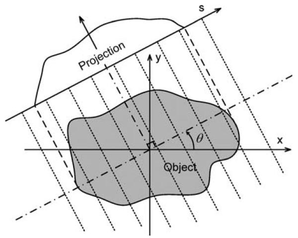
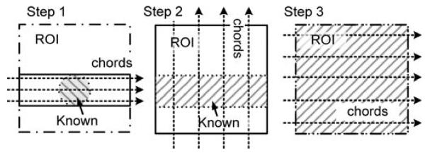
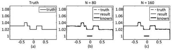
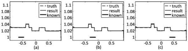
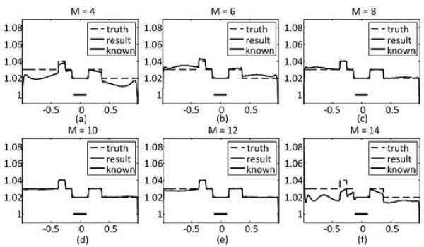
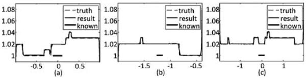
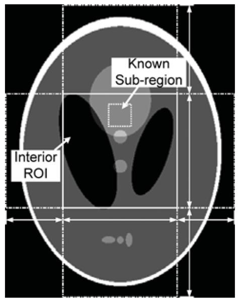
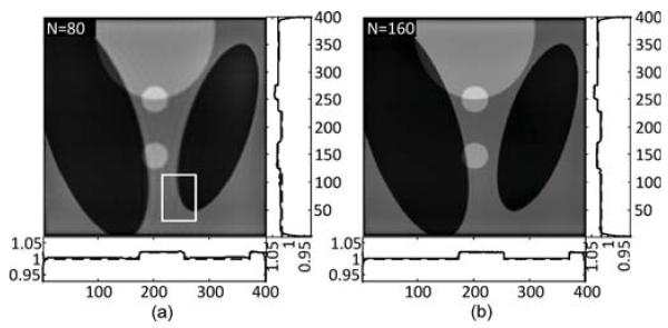
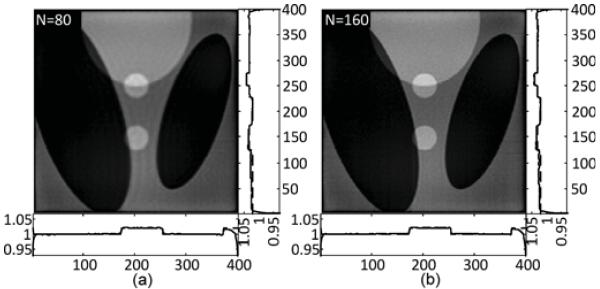
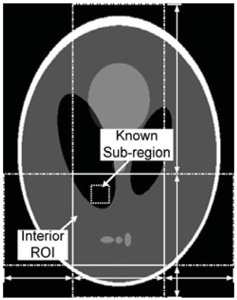
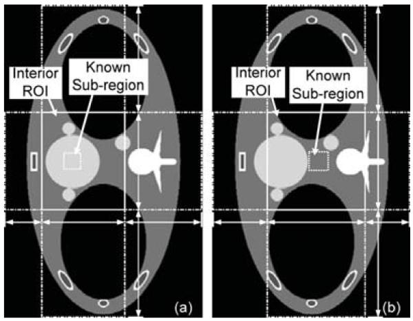
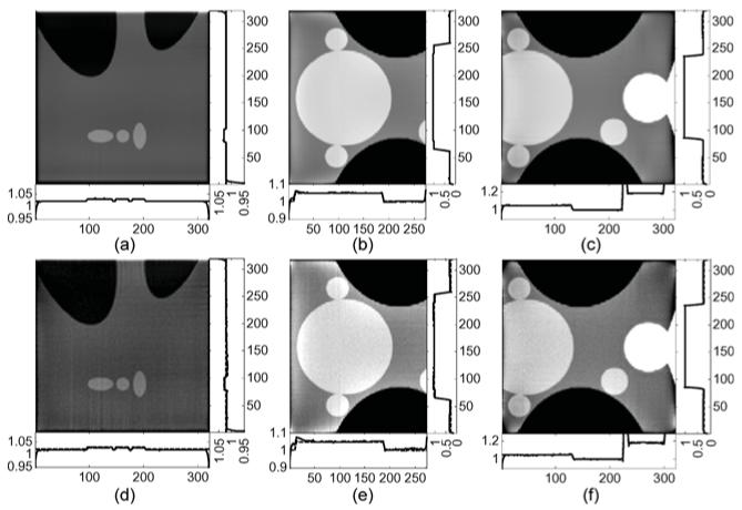
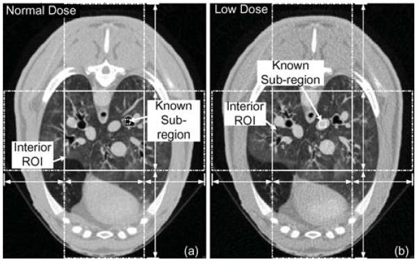
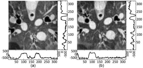
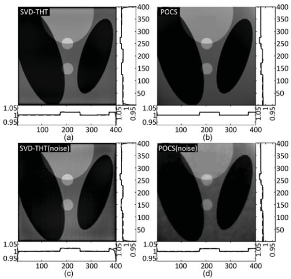
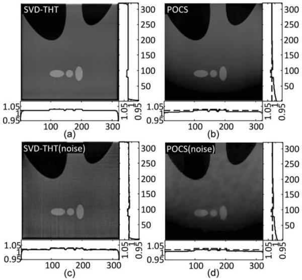
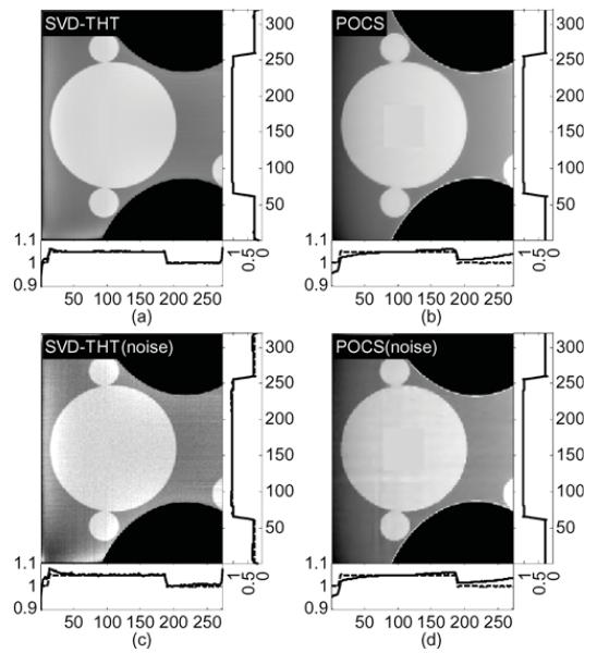
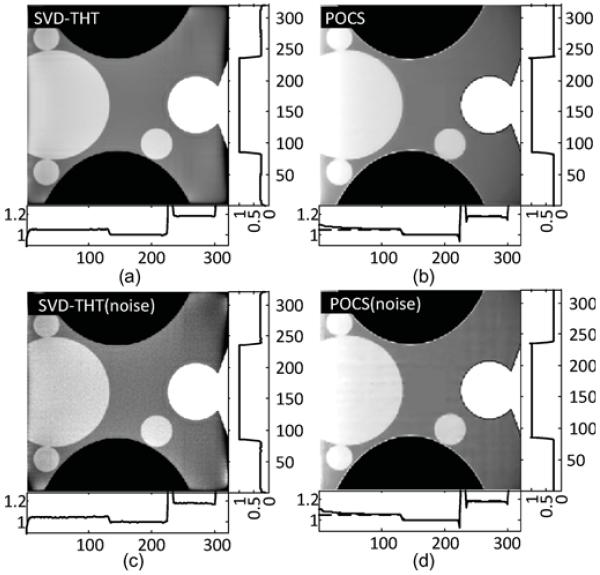
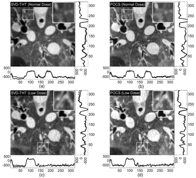
The long-standing interior problem has important mathematical and practical implications. The recently developed interior tomography methods have produced encouraging results. A particular scenario for theoretically exact interior reconstruction from truncated projections is that there is a known sub-region in the ROI. In this paper, we improve a novel continuous singular value decomposition (SVD) method for interior reconstruction assuming a known sub-region. First, two sets of orthogonal eigen-functions are calculated for the Hilbert and image spaces respectively. Then, after the interior Hilbert data are calculated from projection data through the ROI, they are projected onto the eigen-functions in the Hilbert space, and an interior image is recovered by a linear combination of the eigen-functions with the resulting coefficients. Finally, the interior image is compensated for the ambiguity due to the null space utilizing the prior sub-region knowledge. Experiments with simulated and real data demonstrate the advantages of our approach relative to the POCS type interior reconstructions.

Fig. 1

Illustration of projection geometry.

Fig. 2

Illustration of the three-step chord reconstruction scheme.

Fig. 3

The first eight eigen-functions of the Sturm–Liouville problem. The boundary points are a₁ = −2.56, a₂ = −1.0, a₃ = 1.0, and a₄ =2.56.

Fig. 4

Reconstruction results by the SVD-THT without compensation using different number of eigen-functions N. (a) True profile. For (b) and (c) N equals to 80 and 160, respectively.

Fig. 5

Reconstruction results by the SVD-THT with null space compensation using different number of eigen-functions N. (a) True profile. (b) and (c) Compensated profiles with N equals to 80 and 160, respectively. Location of prior known subregion is marked with a bold line segment in each panel.

Fig. 6

Reconstruction results by the SVD-THT with null space compensation using different prior known subregions. From left to right: the known subregions are [−0.35, −0.55], [−0.30, −0.10], and [0.35, 0.55], respectively. The location of prior known subregion is marked with a bold line segment.

Fig. 7

Reconstruction results by the SVD-THT with null space compensation using different number of null space functions M. From (a)–(f) M equals to 4, 6, 8, 10, 12, and 14, respectively. The location of prior known subregion is marked with a bold line segment.

Fig. 8

Reconstruction results by the SVD-THT with null space compensation and different locations of the ROI. The boundary points are a₁ = −2.56, a₂ = −1.0, a₃ = 1.0, and a₄ = 2.56, in (a). In (b) they are a₁ = −2.56, a₂ = −2.0, a₃ = 2.0, and a₄ = 2.56. In (c) they are a₁ = −2.56, a₂ = −2.0, a₃ = 2.0, and a₄ = 2.56. The location of prior known subregion is marked with a bold line segment.

Fig. 9

An interior problem of the Shepp–Logan phantom. The gray scale window is [1.0, 1.05].

Fig. 10

The SVD-THT reconstruction results of the Shepp–Logan phantom from noise-free projections. The number of eigen-functions N is 80 in (a) and 160 in (b). In (a), the white rectangle indicates the subregion to measure the spatial resolution along the ellipsoid edge.

Fig. 11

The SVD-THT reconstruction of the Shepp–Logan phantom from noisy projections. The number of eigen-functions N is set to 80 in (a) and 160 in (b).

Fig. 12

Challenging interior problem on the Shepp–Logan phantom.

Fig. 13

Two interior problems on the FORBILD Thorax phantom. The ROI regions are marked by solid rectangles. The prior known subregions are marked by small dotted rectangles. The horizontal and vertical line segments with arrows indicate the four boundary points for the SVT-THT method. The gray scale window is [0.92, 1.07].

Fig. 14

SVD-THT reconstruction results of the problems defined in Figs. 12 and 13. (a)–(c) Noise-free reconstructions for Fig. 12 and Fig. 13(a) and (b), respectively. (d)–(f) Corresponding reconstructions from noisy data.

Fig. 15

Two interior problems of real datasets from a sheep thorax perfusion study. (a) Normal dose data set and (b) low dose data set. The images are reconstructed by an FBP algorithm from the complete projection data. The gray scale window is [−1000 HU, 320 HU].

Fig. 16

The SVD-THT reconstructions from real CT data corresponding to the interior problems are defined in Fig. 15. The gray scale window is [−1000 HU, 320 HU].

Fig. 17

Reconstruction result comparisons for the Shepp–Logan interior problem defined in Fig. 9.

Fig. 18

Reconstruction result comparisons for the Shepp–Logan interior problem defined in Fig. 12.

Fig. 19

Reconstruction comparisons for the Thorax interior problem defined in Fig. 13(a).

Fig. 20

Reconstruction comparisons for the Thorax interior problem defined in Fig. 13(b).

Fig. 21

Reconstruction comparisons of real sheep thorax study data sets for the interior problems defined in Fig. 15. The gray scale window is set to [−1000, 320] (HU). The images indicated by the dashed rectangles are magnified in the top-right corner to emphasize the difference between the results reconstructed by the SVD-THT and POCS.

References

1. Yu HY, Ye YB, Wang G. “Interior tomography: Theory, algorithms and applications,”; Proc. SPIE; 2008.p. 70780F.
1. Louis AK, Rieder A. “Incomplete data problems in X-ray computerized tomography,”. Numer. Math. 1989;56(4):371–383.
1. Maass P. “The interior Radon transform,”. SIAM J. Appl. Math. 1992;52(3):710–724.
1. Faridani A, Ritman EL, Smith KT. “Local tomography,”. SIAM J. Appl. Math. 1992;52(2):459–484.
1. Katsevich AI, Ramm AG. “New methods for finding values of the jumps of a function from its local omographic data,”. Inverse Probl. 1995;11:1005–1023.
Publication types