A novel approach for choosing summary statistics in approximate Bayesian computation

Abstract

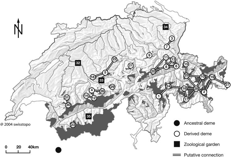
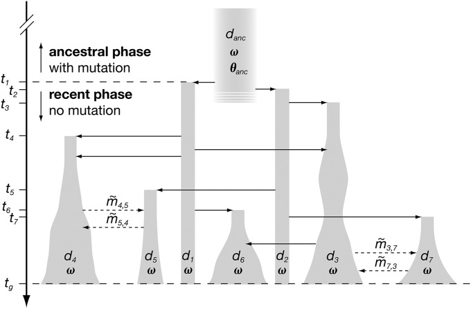
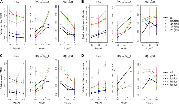
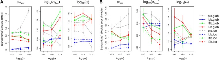
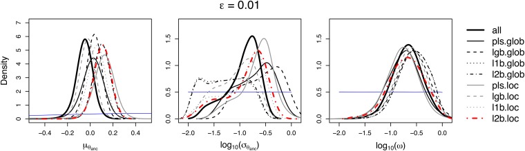
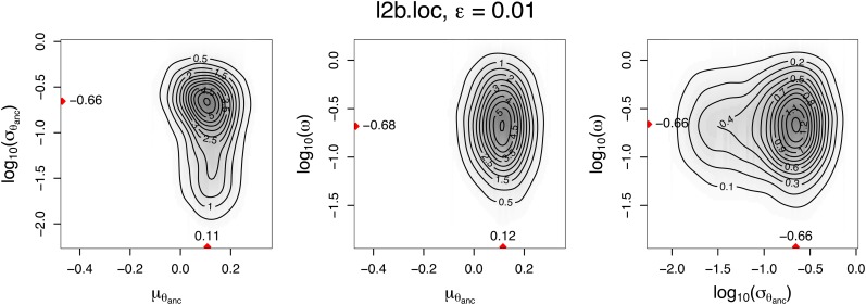
The choice of summary statistics is a crucial step in approximate Bayesian computation (ABC). Since statistics are often not sufficient, this choice involves a trade-off between loss of information and reduction of dimensionality. The latter may increase the efficiency of ABC. Here, we propose an approach for choosing summary statistics based on boosting, a technique from the machine-learning literature. We consider different types of boosting and compare them to partial least-squares regression as an alternative. To mitigate the lack of sufficiency, we also propose an approach for choosing summary statistics locally, in the putative neighborhood of the true parameter value. We study a demographic model motivated by the reintroduction of Alpine ibex (Capra ibex) into the Swiss Alps. The parameters of interest are the mean and standard deviation across microsatellites of the scaled ancestral mutation rate (θ(anc) = 4N(e)u) and the proportion of males obtaining access to matings per breeding season (ω). By simulation, we assess the properties of the posterior distribution obtained with the various methods. According to our criteria, ABC with summary statistics chosen locally via boosting with the L(2)-loss performs best. Applying that method to the ibex data, we estimate θ(anc)≈ 1.288 and find that most of the variation across loci of the ancestral mutation rate u is between 7.7 × 10(-4) and 3.5 × 10(-3) per locus per generation. The proportion of males with access to matings is estimated as ω≈ 0.21, which is in good agreement with recent independent estimates.

Figure 1

Location of Alpine ibex demes in the Swiss Alps. The parts with dark shading represent areas inhabited by ibex. The ancestral deme is located in the Gran Paradiso area in Northern Italy, close to the Swiss border. The two demes in the zoological gardens 33 and 34 were first established from the ancestral one. Further demes, including the two in zoological gardens 32 and 35, were derived from demes 33 and 34. Putative connections indicate the pairs of demes for which migration is considered possible. For a detailed record of the demography and the genealogy of demes see Figure S1 and File S3. For deme names see Table S1. The map was obtained via the Swiss Federal Office for the Environment (FOEN) and modified with permission.

Figure 2

Schematic representation of the demographic model motivated by the reintroduction of Alpine ibex into the Swiss Alps. Shaded shapes represent demes, indexed by d_i, and the width of the shapes reflects the census size. Time goes forward from top to bottom, and the point in time when deme d_i is established is shown as t_i; t_g is the time of genetic sampling. The total time is split by t₁ into an ancestral phase with mutation and a recent phase for which mutation is ignored (see text for details). Solid horizontal arrows represent founder/admixture events and dashed arrows migration. The parameters are (1) the scaled mutation rate in the ancestral deme, θ_anc = 4N_eu; (2) the proportion of males getting access to matings, ω; and (3) forward migration rates between putatively connected demes, ${\tilde{m}}_{i,j}$. The actual model considered in the study contains 35 derived demes (Figure 1 and Table S1). The exact demography is reported in Figure S1 and File S3, transfers.

Figure 3

Accuracy of different methods for choosing summary statistics as a function of the acceptance rate (ε). (A and B) Results for different methods when applied to the whole parameter range (global choice). (C and D) The methods were applied only in the neighborhood of the (supposed) true value (local choice). The performance resulting from using all candidate summary statistics is shown for comparison in both rows. A and C show the root mean integrated squared error (RMISE), relative to the absolute true value. B and D give the absolute error of the posterior median, relative to the absolute true value. Plotted are the medians across n = 500 independent test estimations with true values drawn from the prior (error bars denote the $\text{median}\pm \text{MAD}/\sqrt{n}$, where MAD is the median absolute deviation).

Figure 4

Standardized accuracy of different methods for choosing summary statistics as a function of the acceptance rate (ε). Standaridized¹ means that, before averaging across test sets, we divided the measures of accuracy for the respective method by the measure of accuracy obtained with all candidate summary statistics (this may change the relative order of methods compared to Figure 3, as the average of a ratio is generally not the same as the ratio of two averages). (A) Root mean integrated squared error (RMISE), relative to the RMISE obtained with all summary statistics. (B) Absolute error of the posterior median, relative to the one obtained with all summary statistics. Further details are as in Figure 3.

Figure 5

Marginal posterior distributions inferred from the Alpine ibex data. Posteriors obtained with tolerance ε = 0.01 and various methods for choosing summary statistics are compared. The dot-dashed red line corresponds to the method that performed best in the simulation study (I2b.loc; Tables 2 and 3 and Figures 3 and 4). Thin blue lines give the prior distribution (cf. Table 1). For pairwise joint posterior distributions, see Figure 6. Point estimates and 95% HPD intervals are given in Table 4.

Figure 6

Pairwise joint posterior distributions given data observed in Alpine ibex, obtained with tolerance ε = 0.01 and summary statistics chosen locally via L₂Boosting (l2b.loc). Red triangles denote parameter values corresponding to the pairwise joint modes. Each time, the third parameter has been marginalized over.

References

1. Aeschbacher, A., 1978 Das Brunftverhalten des Alpensteinbocks. Eugen Rentsch Verlag, Erlenbach-Zürich, Switzerland.
1. Akaike H., 1974. A new look at the statistical model identification. IEEE Trans. Automat. Contr. 19: 716–723.
1. Barton N. H., 2000. Genetic hitchhiking. Philos. Trans. R. Soc. B 355: 1553–1562. - PMC - PubMed
1. Beaumont M. A., 2010. Approximate Bayesian computation in evolution and ecology. Annu. Rev. Ecol. Evol. Syst. 41: 379–406.
1. Beaumont M. A., Rannala B., 2004. The Bayesian revolution in genetics. Nat. Rev. Genet. 5: 251–261. - PubMed
Publication types