A reconfigurable NAND/NOR genetic logic gate

Abstract

Background: Engineering genetic Boolean logic circuits is a major research theme of synthetic biology. By altering or introducing connections between genetic components, novel regulatory networks are built in order to mimic the behaviour of electronic devices such as logic gates. While electronics is a highly standardized science, genetic logic is still in its infancy, with few agreed standards. In this paper we focus on the interpretation of logical values in terms of molecular concentrations.

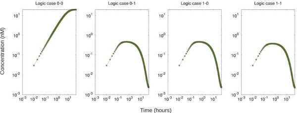
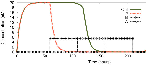
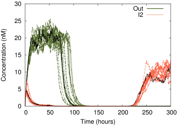
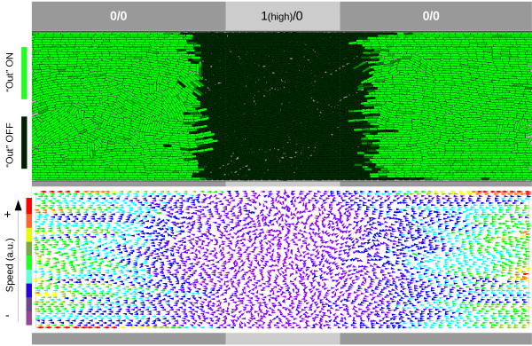
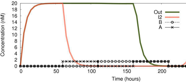
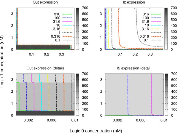
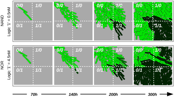
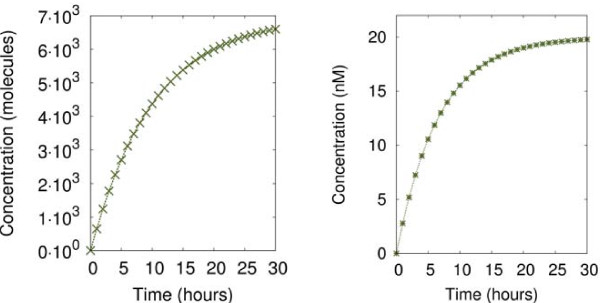
Results: We describe the results of computational investigations of a novel circuit that is able to trigger specific differential responses depending on the input standard used. The circuit can therefore be dynamically reconfigured (without modification) to serve as both a NAND/NOR logic gate. This multi-functional behaviour is achieved by a) varying the meanings of inputs, and b) using branch predictions (as in computer science) to display a constrained output. A thorough computational study is performed, which provides valuable insights for the future laboratory validation. The simulations focus on both single-cell and population behaviours. The latter give particular insights into the spatial behaviour of our engineered cells on a surface with a non-homogeneous distribution of inputs.

Conclusions: We present a dynamically-reconfigurable NAND/NOR genetic logic circuit that can be switched between modes of operation via a simple shift in input signal concentration. The circuit addresses important issues in genetic logic that will have significance for more complex synthetic biology applications.

Figure 1

Proposed genetic circuit. Our circuit is composed of three well differentiated parts: 1) The OR function, with inputs A and B, inducing the expression of X and I₁ by binding to their correspondent promoter; 2) The NOT function, with output I₂, controlled by a constitutive promoter which is repressed by X; 3) A switch, made up of two constitutive promoters which express repressors R₁ and R₂ as well as the reporter Out. Protein complexes C_i are formed by the sequestration of the R_i by I_i.

Figure 2

Static observations of circuit. Four logic cases (combination of two binary inputs) tested with logic “0” fixed at 0 nM and logic “1” at 5 nM (deterministic simulation). Perfect NOR behaviour is observed, as the output Out is only expressed at a high level for the input case 0-0. In the other cases, Out expression is repressed (initially expressed slightly due to initial I₂ concentrations). Axes shown in logarithmic scale for both Time (hours) and Concentration (nM).

Figure 3

Continuous observations of circuit. Deterministic study of the change of Out and I₂ over time, while the four logic cases are introduced dynamically. Until t ≈ 60 both inputs are “0” (case 0-0); from 60 until t ≈ 110 input A is a logic “1” (case 1-0); until t ≈ 160 input A is “0” while input B is “1” (case 0-1); until t ≈ 210 both inputs are 1; from there onwards both inputs come back to “0”. Logic “0” represented by 0 nM, logic “1” by 5 nM.

Figure 4

Continuous observations of circuit, with added noise. Change of Out and I₂ over time while the four logic cases are not homogeneous due to noise in input signals (stochastic inputs). During the case 0-0 (until t ≈ 60) the logic value “0” varies within the range [0…0.05] nM; for the case 1-0 (until t ≈ 110) input A varies within the interval [4.5…5.5] (logic “1”) while input B still varies within the previous interval for a logic “0”; same variation ranges for “0” and “1” during cases 0-1 (until t ≈ 160) and 1-1 (until t ≈ 210); From there, again the case 0-0 but with another definition of logic “0”, varying within the range [0…0.005].

Figure 5

Full stochastic simulation with noise. Stochastic simulation (eleven runs) of the changing behaviour of Out and I₂. All input values and times are taken from Figure 4. All expression products in the system are subject to randomness,with Gaussian noise applied to all concentrations in the integration steps of the equations.

Figure 6

Population-based simulation. Sequential observation of a simulated growing population. The surface on which the cells are growing in contains the inputs with both inputs present in the left half (input logic “1”, established at 1.5 nM for this simulation, as before) and neither input present in the right half (input logic “0”, fixed at 0.0 nM, as before). The output Out is represented as if it were a green fluorescent protein: high expression corresponds to a bright green colour of the cells. The high mobility of cells after 50 and 95 hours (due to there being plenty of free space available) lets us see the graphical pattern produced by the predictive behaviour of the circuit. When the population is very crowded (after 180 hours) the behaviour of the circuit is directly proportional to the surface features. Red circled region: wrong predictions being resolved by changing the direction of the switch. Generation time of cells = 12h.

Figure 7

Effect of cell movement on accuracy. Spatial delay in response due to time spent in changing the direction of the switch. The population is growing from the centre of the longitudinal trap (cells washed out at edges) and the image is taken after 300 hours. The middle sector of the trap (light gray) has only one input (case 1/0) at a high level (4.5nM, which leads to a NOR function), and the remaining area (dark gray) has no input (logic case 0/0). The velocity vector field (lower image) shows the direction and magnitude (colour scheme) of the speeds of every cell at the same time (300 hours).

Figure 8

Continuous observations of circuit with lower concentration for logic “1”. Change of Out and I₂ over time while the four logic cases are being introduced dynamically. Until t ≈ 60 both inputs are “0” (case 0-0); from there until t ≈ 110 input A is a logic “1” (case 1-0); until t ≈ 160 input A is “0” while input B is “1” (case 0-1); until t ≈ 210 both inputs are “1”; from there onwards both inputs come back to “0”. As before, logic “0” represented by 0 nM, but this time logic “1” is represented by 1.5 nM.

Figure 9

Effect of different input concentration values. Surface graphs that explore the behaviour of the circuit for different logic “1” and “0” concentrations. For each pair of logic “0” (x axis) and logic “1” (y axis) the experiments shown in Figures 3 and 8 are performed, and the cumulative values of Out and I₂ over time are recorded. Those values are depicted in two ways: (1) colour surface (greyscale) with a linear scale from 0 to 700 (low precision as mean values are shown for intervals), and (2) contour lines (colour) with a logarithmic scale for detail behaviour. Output values (surface) shown in arbitrary units corresponding to the cumulative value.

Figure 10

Multi-functional behaviour of the circuit. Spatial cell growth simulation shown, where the inputs are embedded in the surface as follows: top-left quadrant has no inputs, top-right quadrant has input A (1-0), bottom-left has only input B (0-1) and bottom-right has both inputs A and B (1-1). Both rows show the expression of Out over time, but for different logic “1” standards: 4.5 nM for a NOR logic function (top) and 0.5 nM for a NAND logic gate (bottom). Logic “0” is 0.0 nM in all simulations. a.u.: arbitrary units. Generation time of cells = 24h.

Figure 11

Repressor concentrations over time. Left graph: Repressor X concentration expressed over time, using the set of equations 2. Right graph: Repressor X concentration expressed over time in a simulation of equation 3.

References

-
- Benner SA, Sismour AM. Synthetic biology. Nat Rev Genet. 2005;6(7):533–43. [ http://www.ncbi.nlm.nih.gov/pubmed/16954140] - PMC - PubMed
- Heinemann M, Panke S. Synthetic biology–putting engineering into biology. Bioinformatics. 2006;22(22):2790–9. doi: 10.1093/bioinformatics/btl469. [ http://www.ncbi.nlm.nih. gov/pubmed/16954140] - DOI - PubMed
- Andrianantoandro E, Basu S, Karig DK, Weiss R. Synthetic biology: new engineering rules for an emerging discipline. Mol Syst Biol. 2006;2:2006.0028. [ http://www.pubmedcentral.nih.gov/articlerender.fcgi? artid=1681505&tool=...] - PMC - PubMed
- Lorenzo VD, Danchin A. Synthetic biology: discovering new worlds and new words. EMBO Reports. 2008;9(9):822–827. doi: 10.1038/embor.2008.159. [ http://www.nature. com/embor/journal/vaop/ncurrent/full/embor2008159.html] - DOI - PMC - PubMed
- Moya A, Krasnogor N, Pereto J, Latorre A. Goethe’s dream. EMBO Reports. 2009;10:S28—S32. [ http://www.nature.com/embor/journal/v10/n1s/ full/embor2009120.html] - PMC - PubMed
Publication types
MeSH terms
LinkOut - more resources
Full Text Sources