A weighted and directed interareal connectivity matrix for macaque cerebral cortex

Abstract

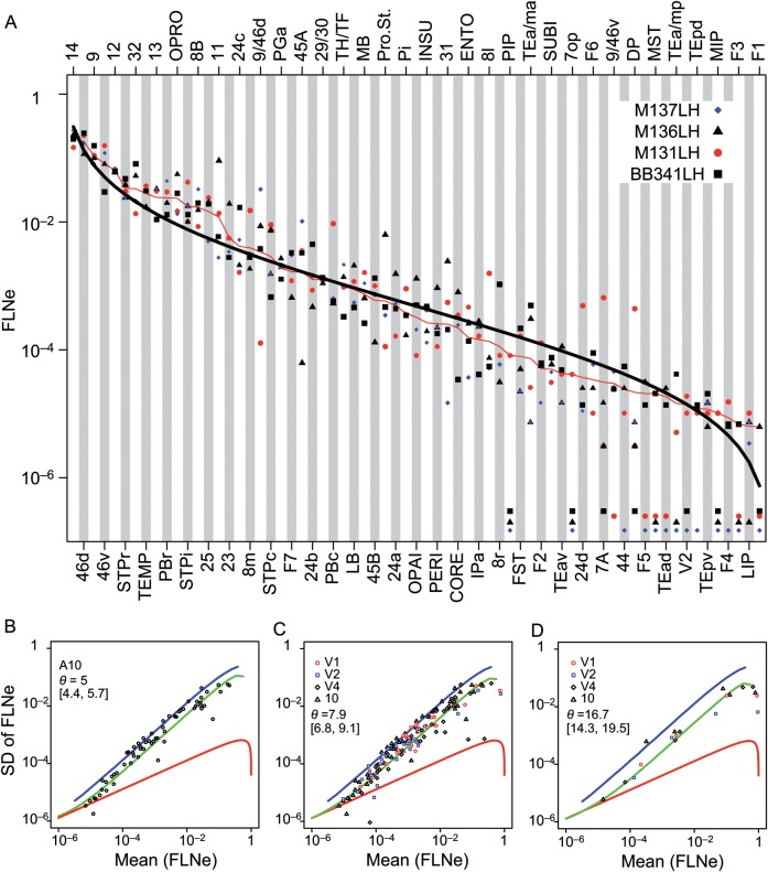
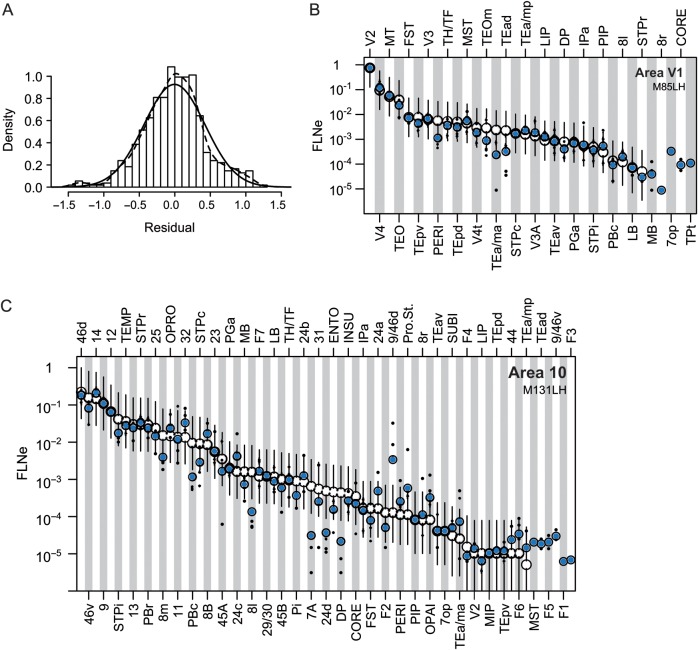
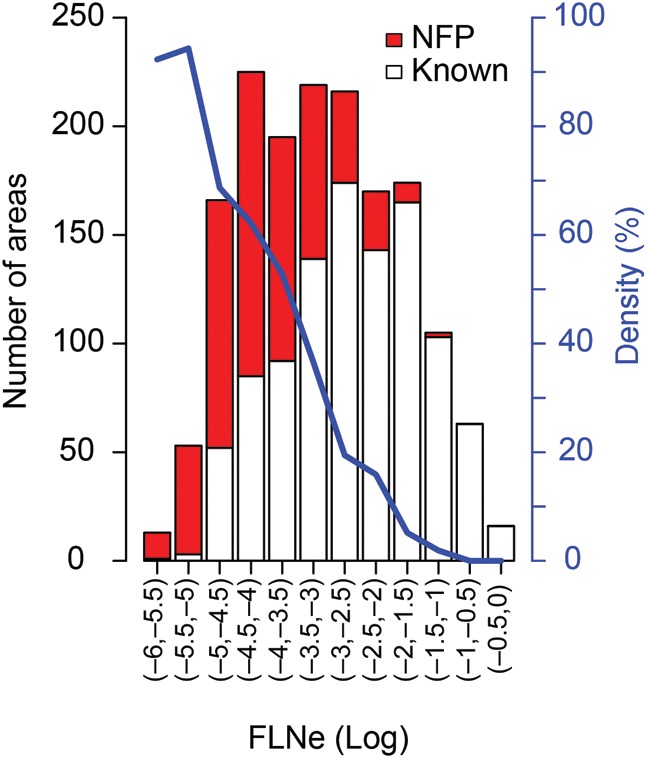
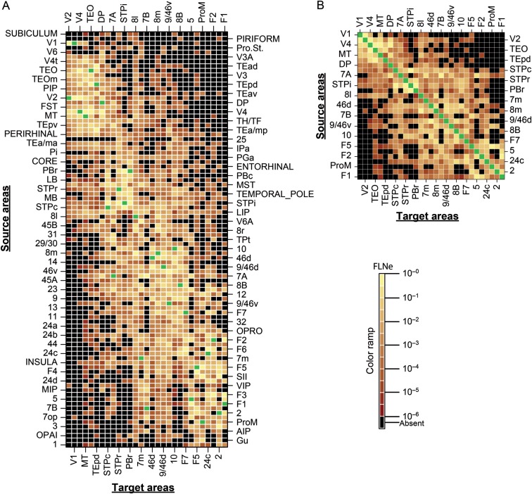
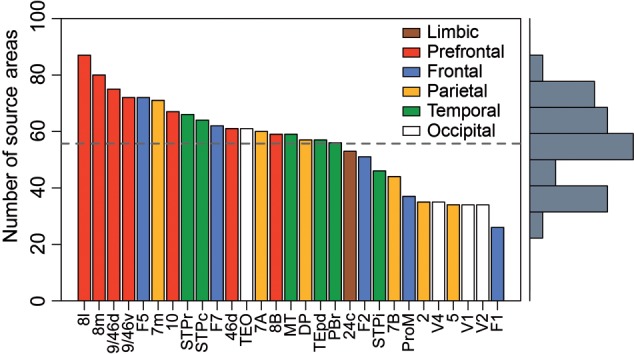
Retrograde tracer injections in 29 of the 91 areas of the macaque cerebral cortex revealed 1,615 interareal pathways, a third of which have not previously been reported. A weight index (extrinsic fraction of labeled neurons [FLNe]) was determined for each area-to-area pathway. Newly found projections were weaker on average compared with the known projections; nevertheless, the 2 sets of pathways had extensively overlapping weight distributions. Repeat injections across individuals revealed modest FLNe variability given the range of FLNe values (standard deviation <1 log unit, range 5 log units). The connectivity profile for each area conformed to a lognormal distribution, where a majority of projections are moderate or weak in strength. In the G29 × 29 interareal subgraph, two-thirds of the connections that can exist do exist. Analysis of the smallest set of areas that collects links from all 91 nodes of the G29 × 91 subgraph (dominating set analysis) confirms the dense (66%) structure of the cortical matrix. The G29 × 29 subgraph suggests an unexpectedly high incidence of unidirectional links. The directed and weighted G29 × 91 connectivity matrix for the macaque will be valuable for comparison with connectivity analyses in other species, including humans. It will also inform future modeling studies that explore the regularities of cortical networks.

Keywords: connection; cortex; graph; monkey; network.

Figure 1.

Surface atlas 3D reconstruction. (A) The 91 areas of the left hemisphere of M132 reconstructed from section drawings (see Supplementary Fig. 7). (B) Lateral and medial views of the 3D anatomical surface displaying areas of M132 transposed on the F99 reference brain medial and lateral view. (C) Inflated F99 right hemisphere surface, displaying the M132 areas registered to it. (D) F99 flat map with representation of the areas of M132. Criteria for parcellation are given in the Materials and Methods section.

Figure 2.

Three-dimensional reconstruction of the 4 injection sites in area 10 (respectively, cases 34, 37, 38, and 39). Injection site in red and white matter in blue. Dotted line shows the limits of area 10. (i) Fronto-lateral view, (ii) frontal view, (iii) fronto-medial view, and (iv) medial view.

Figure 3.

Variability of labeling after repeat injections in area 10. (A) FLNe plotted by area for 4 injections in cortical area 10 ordered by the geometric mean (thin red curve) of the values for each projection (excluding data points for “absent” projections when computing the mean). The thick black curve indicates the expected values for an ordered sample from a lognormal distribution with the same mean and SD. Symbols below 10⁻⁶ indicate zero values. (B–D) The SD as a function of the mean. The curves are the predictions for a Poisson (red), geometric (blue), and the best-fitting negative binomial distribution (green). The dispersion parameter of the negative binomial distribution and its 95% confidence interval are indicated in the inset; (B) values for the 4 injections in area 10; (C) areal values for the repeat injections in V1, V2, V4, and area 10; (D) cumulative regional values.

Figure 4.

Relationships of means and 95% confidence intervals from multiple injections to the values from single injections. (A) Histogram of residuals for multiple injections (V1, V2, V4, and 10) with respect to lognormal order statistics normalized to unit area. Dashed curve: A kernel density estimate of the underlying distribution obtained by convolution of the histogram with a Gaussian; solid curve: Best-fitting normal distribution (mean = −0.003, SD = 0.430). (B) Ordered FLNe values from a single injection in cortical area V1 (white circles) with 95% confidence intervals expected on the basis of a negative binomial distribution (error bars). The small black dots correspond to values obtained from 4 other injections in the same area. The blue circles are the geometric means. For the 3 entries on the far right (MB, 8r, and 7op), there were no labeled neurons from the V1 injection used for FLNe rank ordering. (C) Ordered FLNe values from a single injection in cortical area 10 (white circles) with confidence intervals and small black dots (3 other injections) and blue circles as described for area V1. For the 8 entries on the far right, there were no labeled neurons from the area 10 injection used for FLNe rank ordering.

Figure 5.

Theoretical analysis of projection consistency. (A) Probability of observing zero counts as a function of the true mean for Poisson (red), negative binomial (green), and geometric (blue) distributions. (B) Probability of observing at least one case of zero counts in n injections as a function of the true mean for a negative binomial distribution with dispersion parameter equal to 7.2. (C) Comparison of the probability of observing at least 1 zero as a function of the true mean in n = 5 replications for the geometric (blue) and negative binomial (θ= 7.2) distributions.

Figure 6.

Charts of labeled neurons following injection in area F2. Upper left: Section levels (A–O) indicated on a lateral view of the cortex, red filled region indicates pick-up zone of injection site. (A–O) Charts of coronal sections of retrogradely labeled neurons (red dots). Black rectangle indicates neurons from nearby sections. Blue lettering and asterisk identifies NFP. Red lettering identifies inferred known projections (see text). Scale bar: 2 mm.

Figure 7.

Cortical surface maps for the F2 exemplar injection. Flat map plus medial and lateral inflated maps for injections shown in Figure 8. Connection strengths are encoded as sparse, moderate, or strong (dark to light shades) using green shading for previously reported projections and red for NFP. The area injected is in black.

Figure 8.

Connectivity profiles for 6 injected areas, chosen to illustrate a greater than 3-fold range in number of connections (in-degree distribution, see Fig. 12). The log(FLNe) values are ordered. The solid curves correspond to the predicted order statistics for a lognormal distribution with the same mean and SD as the data. The error bars are 95% confidence intervals, assuming that the data follow a negative binomial distribution with dispersion equal to 7. Connectivity profiles for the remaining injections are displayed in Supplementary Figure 4.

Figure 9.

Weight comparisons for known projections and NFP. Distribution of known projections and NFP as a function of projection magnitude (FLNe) at intervals of 0.5 log₁₀, following the injection of the 29 target areas. Blue line indicates the percentage of NFP within each interval.

Figure 10.

Positive identification of unidirectional pathways. Examples of contiguity of injection site and retrograde labeled neurons in unidirectional pathways. For a unidirectional projection X ≥ Y, we show the labeled neurons in area X following injection in area Y. The injection site in area X is the injection site that failed to label neurons in area Y. Note that the injection site and the reported labeled neurons are in 2 different brains. Scale bars: 2 mm.

Figure 11.

Weighted connectivity matrix. (A) Each row represents 1 of the 91 source areas; each column represents 1 of the 29 injected target areas. The color shows the strength of the projection as indicated by the color bar with black corresponding to absent connections and green for the intrinsic projections that are not included here. The row and column ordering was determined by a clustering algorithm based on similarity of the input and output profiles between areas (see the Materials and Methods section). (B) A weighted connectivity matrix for the 29 × 29 subgraph. For multiple injections, shading is based on geometric mean values.

Figure 12.

In-degree distribution. The number of areas projecting to each of the target areas of this study. Horizontal dashed line indicates the mean in-degree 57.4.

References

1. Adachi Y, Osada T, Sporns O, Watanabe T, Matsui T, Miyamoto K, Miyashita Y. Functional connectivity between anatomically unconnected areas is shaped by collective network-level effects in the macaque cortex. Cereb Cortex. 2012;22:1586–1592. - PubMed
1. Aflalo TN, Graziano MS. Organization of the macaque extrastriate visual cortex re-examined using the principle of spatial continuity of function. J Neurophysiol. 2011;105:305–320. - PMC - PubMed
1. Barabasi AL, Albert R. Emergence of scaling in random networks. Science. 1999;286:509–512. - PubMed
1. Barbas H, Hilgetag CC, Saha S, Dermon CR, Suski JL. Parallel organization of contralateral and ipsilateral prefrontal cortical projections in the rhesus monkey. BMC Neurosci. 2005;6:32. - PMC - PubMed
1. Barbas H, Pandya DN. Architecture and frontal cortical connections of the premotor cortex (area 6) in the rhesus monkey. J Comp Neurol. 1987;256:211–228. - PubMed
Publication types