A critical reevaluation of the stationary axonal cytoskeleton hypothesis

Abstract

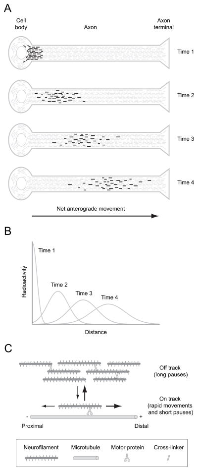
Neurofilaments are transported along axons in a rapid intermittent and bidirectional manner but there is a long-standing controversy about whether this applies to all axonal neurofilaments. Some have proposed that only a small proportion of axonal neurofilaments are mobile and that most are deposited into a persistently stationary and extensively cross-linked cytoskeleton that remains fixed in place for many months without movement, turning over very slowly. In contrast, others have proposed that this hypothesis is based on a misinterpretation of the experimental data and that, in fact, all axonal neurofilaments move. These contrary perspectives have distinct implications for our understanding of how neurofilaments are organized and reorganized in axons both in health and disease. Here, we discuss the history and substance of this controversy. We show that the published data on the kinetics and distribution of neurofilaments along axons favor a simple "stop and go" transport model in which axons contain a single population of neurofilaments that all move in a stochastic, bidirectional and intermittent manner. Based on these considerations, we propose a dynamic view of the neuronal cytoskeleton in which all neurofilaments cycle repeatedly between moving and pausing states throughout their journey along the axon. The filaments move infrequently, but the average pause duration is on the order of hours rather than weeks or months. Against this fluid backdrop, the action of molecular motors on neurofilaments can have dramatic effects on neurofilament organization that would not be possible if the neurofilaments were extensively cross-linked into a truly stationary network.

Figure 1. Axonal transport of neurofilaments

A. Schematic diagram illustrating the movement of a pulse of radiolabeled neurofilaments along an axon in a radio-isotopic pulse labeling experiment, meant to be representative of axons in a long nerve such as the sciatic. To perform such an experiment, radioactive amino acids are injected into the vicinity of neuronal cell bodies. The radiolabeled amino acids become incorporated into newly synthesized proteins, generating a pulse of radiolabeled proteins that move out along the axons by the mechanisms of axonal transport. The most commonly used injection sites are the dorsal root ganglia, which labels sensory neurons, the anterior horn of the spinal cord, which labels motor neurons, and the eye, which labels retinal ganglion cells. This diagram shows a single axon but in reality these experiments are performed on nerves that contain thousands of axons that run in parallel, so the actual kinetics are a summation of the kinetics of many individual axons. The pulse of radiolabeled neurofilaments is sharp initially but spreads considerably over time due to the stochastic, intermittent and bidirectional nature of the movement. B. Schematic illustrating the distribution of the pulse of radiolabeled neurofilaments at the four time points shown in A. The neurofilaments form a symmetrical and slowly moving Gaussian wave that spreads as it propagates distally (Brown et al. 2005; Craciun et al. 2005; Hoffman et al. 1985; Hoffman and Lasek 1975; Hoffman et al. 1983; Jung and Brown 2009; Xu and Tung 2001). The average velocity is usually in the range 0.2–1.0 mm/day and depends on the age of the animal and the particular nerve being studied. C. Schematic diagram of the “stop and go” model of neurofilament transport. Neurofilaments are transported by motor proteins along microtubule tracks in a rapid intermittent manner, cycling between kinetically distinct on-track and off-track states. Neurofilaments in the on-track state engage in rapid bouts of movement interrupted by short pauses, whereas neurofilaments in the off-track state pause for prolonged periods without any movement. Off-track neurofilaments may be interconnected temporarily by cytoskeletal cross-linkers such as spectraplakins. The neurofilaments switch between forwards (anterograde) and backwards (retrograde) movement, but anterograde movements predominate, resulting in a net anterograde directionality.

Figure 2. Contamination of the neurofilament transport kinetics in mouse optic nerve by Slow Component ‘b’ proteins

A. Schematic diagram of hypothetical radiolabeled axonal proteins resolved by one dimensional (1D) gel electrophoresis, i.e. sodium dodecyl sulfate polyacrylamide gel electrophoresis (SDS-PAGE), or two dimensional (2D) gel electrophoresis, i.e. isoelectric focusing (IEF) in the first (horizontal) dimension and SDS-PAGE in the second (vertical) dimension. Slow Component ‘a’ proteins (which are relatively few) are shown in red and Slow Component ‘b’ proteins (which are relatively numerous) are shown in green. The box demarcated with the dashed line shows a hypothetical Slow Component ‘a’ protein, Protein A, and a hypothetical Slow Component ‘b’ protein of similar molecular mass, Protein B. These proteins comigrate using 1D electrophoresis, but can be resolved using 2D electrophoresis because they have different isoelectric points. B. Schematic representation of the distribution of a pulse of these radiolabeled proteins along a hypothetical short nerve (meant to be representative of the optic nerve) at three different time points. Radioactivity associated with Protein A, which moves more slowly (in Slow Component ‘a’), is shown in red. Radioactivity associated with Protein B, which is transported more rapidly (in Slow Component ‘b’), is shown in green. The dashed black line represents the sum of the radioactivity profiles for the two proteins and is representative of the profile that would be observed if the analysis was performed using 1D electrophoresis of total nerve protein, as in Nixon & Logvinenko (1986). C. Schematic representation of the time course of appearance and disappearance of radioactive protein in the entire nerve window over time. Note that Protein B, which moves in Slow Component ‘b’, enters and exits the nerve window more rapidly than Protein A. The decay kinetics of the individual proteins are monophasic, but the decay kinetics of the two proteins combined (dashed black line) is biphasic. The initially more rapidly declining phase corresponds to Protein B, which departs the nerve more rapidly, and the later more slowly declining phase corresponds to Protein A, which departs more slowly. D. The experimental data of Nixon and colleagues, as plotted in Li et al. (2012). The symbols represent the data for neurofilament protein M from Yuan et al. (2009) (open squares) and from Nixon & Logvinenko (1986) (open circles). Yuan et al. (2009) used a Triton-insoluble protein fraction, yielding pure neurofilament protein and monophasic decay kinetics. In contrast, Nixon & Logvinenko (1986) used total nerve protein (soluble and insoluble), yielding biphasic decay kinetics. The solid black line represents the output of the model, assuming contamination of the neurofilament protein kinetics with a hypothetical Slow Component ‘b’ protein (relative weighting of 60% neurofilament protein and 40% Slow Component ‘b’ protein). Note that the model shows good agreement with the biphasic decay kinetics of Nixon & Logvinenko (1986) at all times, and also with the monophasic decay kinetics of Yuan et al. (2009) at later times (>50 days), after the Slow Component ‘b’ proteins in the model have left the nerve window. Thus the biphasic decay kinetics of Nixon & Logvinenko (1986) can be explained by contamination of the neurofilament transport kinetics with faster moving Slow Component ‘b’ proteins.

Figure 3. Computational modeling of neurofilament transport in the mouse optic nerve

A. Schematic of the optic pathway from one eye. The axons of retinal ganglion cells course through the retina and emerge from the eye at the optic disk to form the optic nerve, which extends to the contralateral side of the brain. B. The gradient in neurofilament content along the mouse optic nerve. The experimental data (open circles) are from Nixon & Logvinenko (1986). The solid line represents the predictions of our computational model (from Li et al. 2012). C. The gradient in average neurofilament transport velocity that is required to explain the gradient in neurofilament content shown in B (from Li et al. 2012). D. The kinetics of neurofilament transport in the mouse optic nerve (from Li et al. 2012). The open symbols represent the experimental data from Yuan et al. (2009) for NFL and NFM, recalculated as described in Li et al. (2012), and the solid line represents the output of the “stop and go” model. The radioactivity at each time point is expressed as a percentage of the total radioactivity in the nerve window at day 10, as described in Li et al. (2012). Note that the model generates a symmetrical wave when the kinetic parameters are uniform (Brown et al. 2005; Craciun et al. 2005; Jung and Brown 2009), but the wave here is not perfectly symmetrical because of the gradient in the transport velocity.

References

1. Ackerley S, Thornhill P, Grierson AJ, Brownlees J, Anderton BH, Leigh PN, Shaw CE, Miller CC. Neurofilament heavy chain side arm phosphorylation regulates axonal transport of neurofilaments. Journal of Cell Biology. 2003;161(3):489–95. - PMC - PubMed
1. Alami NH, Jung P, Brown A. Myosin Va increases the efficiency of neurofilament transport by decreasing the duration of long-term pauses. Journal of Neuroscience. 2009;29(20):6625–34. - PMC - PubMed
1. Baas PW, Brown A. Slow axonal transport: the polymer transport model. Trends in Cell Biology. 1997;7(10):380–384. - PubMed
1. Barry DM, Millecamps S, Julien JP, Garcia ML. New movements in neurofilament transport, turnover and disease. Experimental Cell Research. 2007;313(10):2110–20. - PubMed
1. Black MM, Lasek RJ. Axonal transport of actin: slow component b is the principal source of actin for the axon. Brain Research. 1979;171(3):401–13. - PubMed
Publication types
Substances
LinkOut - more resources