Population response to natural images in the primary visual cortex encodes local stimulus attributes and perceptual processing

Abstract

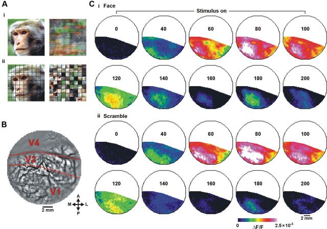
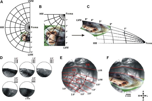
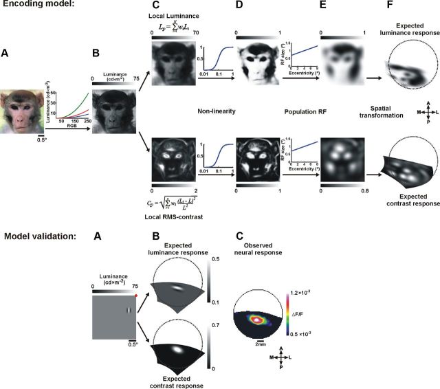
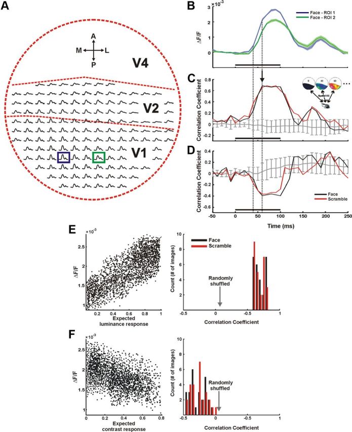
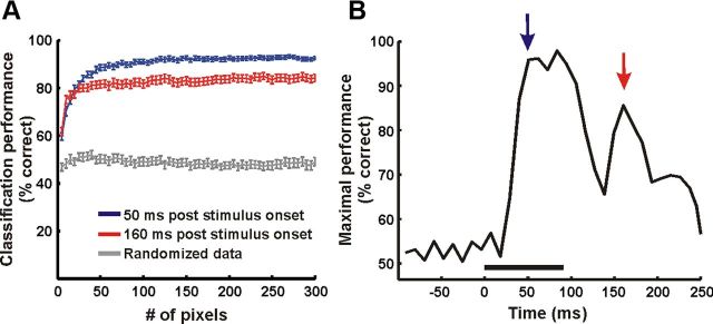
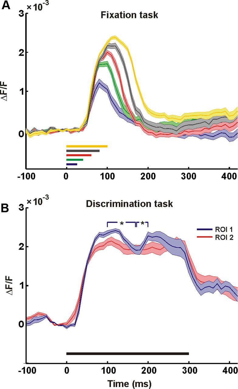
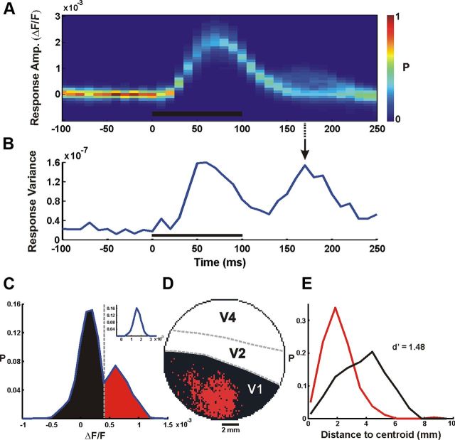
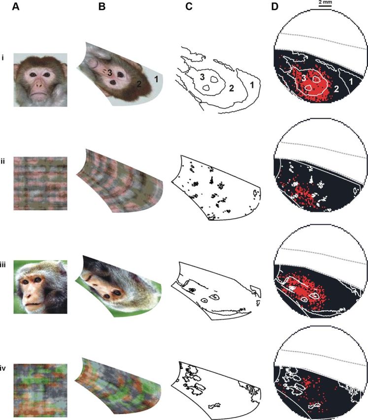
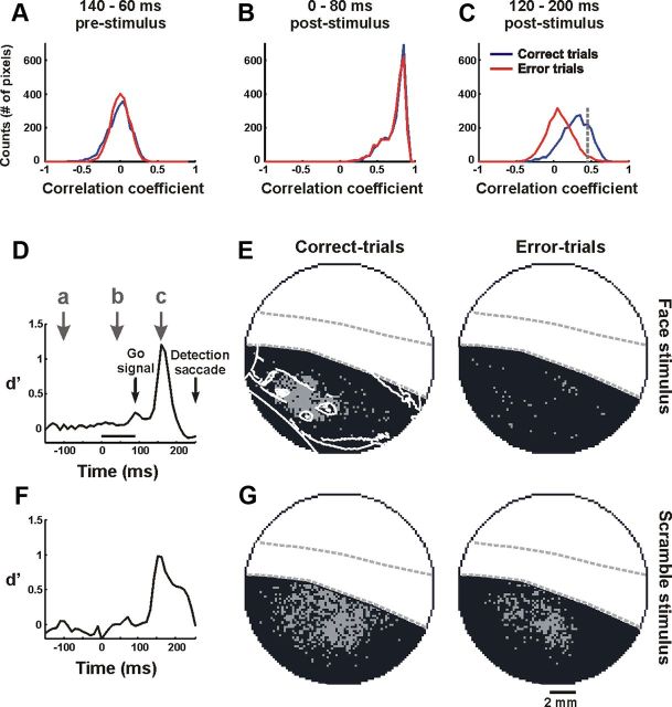
The primary visual cortex (V1) is extensively studied with a large repertoire of stimuli, yet little is known about its encoding of natural images. Using voltage-sensitive dye imaging in behaving monkeys, we measured neural population response evoked in V1 by natural images presented during a face/scramble discrimination task. The population response showed two distinct phases of activity: an early phase that was spread over most of the imaged area, and a late phase that was spatially confined. To study the detailed relation between the stimulus and the population response, we used a simple encoding model to compute a continuous map of the expected neural response based on local attributes of the stimulus (luminance and contrast), followed by an analytical retinotopic transformation. Then, we computed the spatial correlation between the maps of the expected and observed response. We found that the early response was highly correlated with the local luminance of the stimulus and was sufficient to effectively discriminate between stimuli at the single trial level. The late response, on the other hand, showed a much lower correlation to the local luminance, was confined to central parts of the face images, and was highly correlated with the animal's perceptual report. Our study reveals a continuous spatial encoding of low- and high-level features of natural images in V1. The low level is directly linked to the stimulus basic local attributes and the high level is correlated with the perceptual outcome of the stimulus processing.

Figure 1.

Spatiotemporal activation pattern of the VSDI signal. A, Example of a stimulus pair (monkey's face and its scrambled versions). Ai, scrambling using phase perturbations; Aii, segment scrambling (see Materials and Methods). B, Image of the blood vessel patterns of the exposed cortex. Dashed red lines mark the borders between V1 and V2 and the lunate sulcus. C, VSDI activation map evoked over V1 by 100 ms presentation of visual stimulus. Ci, ii, Show a sequence of frames evoked by the presentation of a coherent face stimulus and a scramble face stimulus (segment scrambling), respectively. Maps are averaged over 28 trials. Numbers correspond to milliseconds after stimulus onset. A, anterior; P, posterior; M, medial; L, lateral.

Figure 2.

Analytical 2D mapping of the visual stimuli onto cortical space. A, An example of a stimulus as seen in the visual field, shown here against a polar grid. B, Enlargement of the stimulus zone in A. C, The stimulus zone in B after applying the analytical spatial transformation. D, Top, A series of intrinsic imaging activation patterns evoked by a vertical bar (0.25 × 6°) separately presented at different locations parallel to the LVM: LVM −0.5°, LVM −1.5°, VM −2.5° (−, to the left of LVM in the contralateral hemifield). Bottom, A series of activation patterns evoked by a horizontal bar (6 × 0.25°) separately presented parallel to the HM: HM −2.5°, HM −3.5° (−, below HM). Insets, Stimulus positions relative to the fixation point (red dot). E, Image of the blood vessel pattern in V1 taken on one VSDI experiment. The solid red lines mark the retinotopic mapping of the Cartesian lines shown in D. Dashed red lines, the borders between V1 and V2 and the LUS; black asterisks, two anchor points used for image registration; black dots, six points for optimizing the model's fit (see Materials and Methods; note, the intrinsic imaging recording and the VSDI recording were done on separate imaging days, therefore due to the relative angle between the camera and the cortical surface the blood vessels may seem slightly shifted between D and E). F, The spatially transformed stimulus (from C) after image registration on the exposed cortical surface. LUS, lunate sulcus; UVM, upper vertical meridian; LVM, lower vertical meridian; HM, horizontal meridian, A, anterior; P, posterior; M, medial; L, lateral.

Figure 3.

Computing the expected neural response. Top, A, Example of a visual stimulus. B, The stimulus in A after conversion of each pixel from RGB to luminance values (maximum luminance of the screen = 75 cd × m⁻²). C, The local luminance (above) and local RMS-contrast (below) obtained by the weighted sum of a circular patch with a radius of 0.15°. D, The stimulus luminance and RMS-contrast shown in C, operated on by a nonlinear function (Naka–Rushton). E, The expected luminance response (above) and the expected contrast response (below) obtained by the weighted sum of a circular population RF (with size that varied linearly as a function of eccentricity). F, The expected luminance and contrast response after spatial transformation to cortical coordinates of V1 (Fig. 2; see Materials and Methods). Bottom, Model validation. Computing the expected neural response of a single Gabor stimulus. A, A Gabor element presented over a gray background. The red dot represents the fixation point of the monkey. B, The expected luminance and contrast response of a single Gabor, after spatial transformation to cortical coordinates (calculated as described above). C, The neural population response evoked in V1 by the presentation of a single Gabor, averaged over two time frames at 60–70 ms poststimulus onset (shown after 2D Gaussian filter with σ = 1.5 pixels). The spatial correlation values between the expected and the observed response are 0.58, 0.83 for the local luminance and local contrast, respectively, calculated over 452 pixels.

Figure 4.

Spatial correlation between the maps of the population response and the expected response. A, Neural response time course along the imaged cortical space evoked by a face stimulus. Each plot corresponds to the mean signal averaged over 1 × 1 mm² (6 × 6 pixels). Dashed red lines schematically mark borders between cortical regions. B, Enlargement of the signals averaged over the region of interest (ROI) in the blue and green boxes in B. Trace width denotes ±1 SEM over 28 trials; the black bar represents the stimulus presentation time. C, D, Typical example of spatial correlation between the neural response (spread over 2034 pixels in V1) and cortical mapping of the expected luminance response (C) and the expected contrast response (D) as a function of time (see Materials and Methods). Black and red lines correspond to a coherent face stimulus (shown in A and B) and a scramble stimulus, respectively. Gray curve, correlation between the measured neural activity and the expected activity computed on a randomly shuffled set of stimuli (mean ± SD, n = 50). Dashed gray lines, the first time point exhibiting significant correlation and the time point with maximal correlation. Black bar denotes stimulus presentation. E, Left, Shows an example of a scatter plot of the expected luminance response of one face stimulus versus the neural response of all the pixels in V1 during one frame (t = 60 ms after stimulus onset, marked with an arrow in D, r = 0.69). Right, Shows the histogram of the spatial correlation values of all the images presented to both monkeys (n_face = 26, n_scramble = 26, scrambled images include both types of scrambling) at t = 60 ms after stimulus onset. No significant difference was found between the face and scramble. F, Same as in E, only for the correlation between the expected contrast response and the neural response (r = −0.39).

Figure 5.

Single-trial readout performance. A, Performance of an SVM classifier (see Materials and Methods) at the single trial level as a function of the number of pixels used (example of one imaging session, n = 56 trials, 28 face trials, 28 segment scrambling nonface trials). Blue and red traces, Classification performance using neural activity at t = 50 ms and t = 160 ms after stimulus onset, respectively (mean ± SEM, n = 50 iterations, face vs phase perturbation nonface). Gray trace, Performance of the classifier trained with the randomized trial category (control). B, Maximal performance of the classifier over time (using 125 pixels), showing two phases of information processing. Blue and red arrows mark the time frames plotted in A.

Figure 6.

An off-response cannot explain the late neuronal modulation. A, Time course of responses evoked by a scramble stimulus with variable duration in a fixation task (i.e., a naive monkey was required to fixate without the report about the stimulus category), averaged over 227 pixels in the center of the chamber. Colors denote the stimulus duration time: blue, green, red, gray, and yellow correspond to 25, 40, 60, 80, and 100 ms, respectively. Line width denotes ±1 SEM over 15 trials. B, Time course of responses evoked by a 300 ms stimulus presentation in a face/scramble discrimination task, averaged over 172 and 181 pixels in two separate regions of interests (ROIs). Line width denotes ±1 SEM over five trials (carefully checked for eye movements); black bar, stimulus presentation. The blue ROI exhibits significant modulation (Wilcoxon rank-sum test between t = 100 and t = 170 ms poststimulus onset, p < 0.005 and between t = 170 and t = 200 ms poststimulus onset, p < 0.005).

Figure 7.

Spatial mapping of the late response. A, Example of VSDI amplitude distribution across V1 pixels as a function of time (one face stimulus imaging session, averaged over 30 trials, n = 2510 pixels, bin width = 10 ms). Color bar denotes normalized distribution; black bar denotes stimulus presentation time. B, The variance of the VSDI response across all V1 pixels, i.e., the spatial variance, as a function of time. C, Bimodal distribution in VSDI amplitude at time marked with arrow in B (t = 170 ms after stimulus onset). Dashed gray line marks the amplitude threshold for the mapping in D. Inset shows a unimodal amplitude distribution at t = 60 ms after stimulus onset. D, Neural activity map in V1 at t = 170 ms after stimulus onset. Black and red pixels are those below and above amplitude threshold, respectively. E, Distributions of distance-to-centroid of the black and red pixel groups in D.

Figure 8.

Linking the late neural response with stimulus features. Four stimuli superimposed over the map of V1 activity. A, Stimuli. B, Stimuli after spatial transformation. C, Contour line of the stimuli after spatial transformation (defined using a standard algorithm for edge detection for presentation purpose only). D, Contour line of the stimuli superimposed on the late response mapping after threshold crossing (as shown in Fig. 7; on each row the neural activity was averaged over 30 trials). 1, Area with maximal luminance of the image but located outside the face region. 2, Area with low luminance. 3, Area with high luminance inside the face region. Stimuli (i) and (ii) were positioned at x = 1.9°, y = 3.7° from the fovea (center of image), stimuli (iii) and (iv) at x = 1.8°, y = 3.7° from the fovea.

Figure 9.

Error trials analysis. A–C, Distribution of the temporal correlation coefficient, r, (see Materials and Methods) in face stimulus trials, averaged over the correct trials (blue, n = 7) and the error trials (red, n = 7) in one recording session. For adequate comparison, we matched the number of correct and error trials. The distributions are shown before stimulus onset (A), during the early response (B), and during the late response (C). Temporal correlations were calculated in a window of 80 ms. D, Distance between the correct and the error histograms (d′) as a function of time. Note the time scale denotes the center of the time window used to calculate the temporal correlations. Arrows, Time points corresponding to the distributions in A–C. E, Map of all the pixels in V1 with r value above (gray pixels) and below threshold (black pixels). Threshold is marked by the dashed gray line in C. Left and right show the correct and the error trials, respectively. F, G, As in D and E, only for scramble stimulus trials (segment scrambling; n = 7 correct trials and 7 error trials). The data here were obtained from a single recording session.

References

1. Albrecht DG, Hamilton DB. Striate cortex of monkey and cat: contrast response function. J Neurophysiol. 1982;48:217–237. - PubMed
1. Albrecht DG, Geisler WS, Crane AM. Nonlinear properties of visual cortex neurons: temporal dynamics, stimulus, selectivity, neural performance. In: Chalupa LM, Werner JS, editors. The visual neurosciences. Cambridge: MIT; 2004. pp. 747–764.
1. Angelucci A, Levitt JB, Walton EJ, Hupe JM, Bullier J, Lund JS. Circuits for local and global signal integration in primary visual cortex. J Neurosci. 2002;22:8633–8646. - PMC - PubMed
1. Arieli A, Grinvald A, Slovin H. Dural substitute for long-term imaging of cortical activity in behaving monkeys and its clinical implications. J Neurosci Methods. 2002;114:119–133. - PubMed
1. Ayzenshtat I, Meirovithz E, Edelman H, Werner-Reiss U, Bienenstock E, Abeles M, Slovin H. Precise spatiotemporal patterns among visual cortical areas and their relation to visual stimulus processing. J Neurosci. 2010;30:11232–11245. - PMC - PubMed
Publication types
LinkOut - more resources