Denoising MR spectroscopic imaging data with low-rank approximations

Abstract

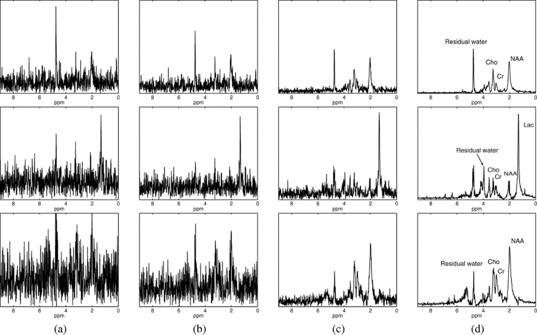
This paper addresses the denoising problem associated with magnetic resonance spectroscopic imaging (MRSI), where signal-to-noise ratio (SNR) has been a critical problem. A new scheme is proposed, which exploits two low-rank structures that exist in MRSI data, one due to partial separability and the other due to linear predictability. Denoising is performed by arranging the measured data in appropriate matrix forms (i.e., Casorati and Hankel) and applying low-rank approximations by singular value decomposition (SVD). The proposed method has been validated using simulated and experimental data, producing encouraging results. Specifically, the method can effectively denoise MRSI data in a wide range of SNR values while preserving spatial-spectral features. The method could prove useful for denoising MRSI data and other spatial-spectral and spatial-temporal imaging data as well.

Fig. 1

Simulation results of LP-based low-rank filtering with and without Hankel constraint: (a) original (red) and noisy (black) spectra at low (I) and high (II) noise levels; (b) and (d) denoised spectra with Hankel constraint (Cadzow) for L₂ = 20 and 8, respectively; (c) and (e) denoised spectra without Hankel constraint (step 2 of LORA) for L₂ = 20 and 8, respectively. Note that the Hankel constraint helped reduce noise but at the expense of spectral artifacts.

Fig. 2

Monte Carlo study of rank L₂ selection based on AIC: top row shows the mean AIC value (averaged over 256 noise realizations) as a function of L̂₂ at (a) low noise level with SNR_e=26.61 dB and SNR_p=94.4; (b) medium noise level with SNR_e=17.03 dB and SNR_p=30.4; (c) high noise level with SNR_e=12.76 dB and SNR_p=17.9. The true rank L₂ in this experiment was 20.

Fig. 3

Denoising results—spatial distributions ρ(r, f₁) at a SNR frequency [3.94 ppm; see Fig. 5(f)] obtained from (a) noisy data; (b) LORA denoising; (c) wavelet denoising; (d) sparse 3-D transform-domain collaborative filtering; (e) Gaussian apodization; and (f) noiseless data. Corresponding errors of (b)–(e) are shown in (g)–(j), respectively.

Fig. 4

Denoising results—spatial distributions ρ(r, f₂) at a low-SNR frequency [6.66 ppm; see Fig. 5(f)], obtained from (a) noisy data; (b) LORA denoising; (c) wavelet denoising; (d) sparse 3-D transform-domain collaborative filtering; (e) Gaussian apodization; and (f) noiseless data. Corresponding errors of (b)–(e) are shown in (g)–(j), respectively.

Fig. 5

Denoising results—spectra at a particular voxel, marked as “1” in Fig. 3(f), obtained from (a) noisy data; (b) LORA denoising; (c) wavelet shrinkage; (d) sparse 3-D transform-domain collaborative filtering; (e) Gaussian apodization; and (f) noiseless data. Corresponding errors of (b)–(e) are shown in (g)–(j), respectively. All spectra are shown in the real-valued mode.

Fig. 6

Noise reduction factor g for low-rank filtering based on partial separability as a function of the estimated rank L̂₁. Empirical values of g (black) and corresponding theoretical approximations (red) were computed according to (18) and (19), respectively. The true rank L₁ = 8. Notice that in the region L̂₁ > L₁, the theoretically predicted values of g tend to its empirical values and both approach 1 in the full-rank case.

Fig. 7

Monte Carlo study of low-rank filtering based on partial separability: (a) representative noisy and denoised spectra at three SNR levels; (b) error distributions calculated as the histograms of e and ē according to (21) at a particular location (r₀, f₀). For this illustrative example, r₀ is a representative voxel in the white matter region marked as “2” in Fig. 3(e) and f₀ is the frequency point marked in Fig. 7(a). Notice the reduced noise variances achieved by denoising.

Fig. 8

Monte Carlo study of low-rank filtering based on linear predictability: (a) representative noisy and denoised spectra at three noise levels; (b)–(d) error distributions calculated as the histograms of e and ē according to (21) at particular locations (r₀, f₁), (r₀, f₂), and (r₀, f₃), respectively. For this illustrative example, r₀ is a representative voxel in the white matter region marked as “2” in Fig. 3(f) and f₁, f₂, and f₃ are the frequency points marked in Fig. 8(a). Notice that the denoising performance is frequency dependent.

Fig. 9

Denoising results from in vivo experimental data. Spatial distributions corresponding to NAA in the region from 1.9 to 2.1 ppm (top row), Lac in the region from 1.2 to1.37 ppm (middle row), and Glx in the region from 2.7 to 2.8 ppm (bottom row) obtained from (a) noisy data; (b) spatial denoising; (c) PS-based low-rank filtering; (d) LP-based low-rank filtering of the results in (c) (the final output of LORA).

Fig. 10

Denoising results from in vivo experimental dataset: spectra at three voxels in the region outside of electrocogualation (voxel 1, top row, and voxel 3, bottom row) and inside of electrocogualation area (voxel 2, middle row), obtained from (a) noisy data; (b) spatial denoising; (c) PS-based low-rank filtering of the spatial filtering results; (d) LP-based low-rank filtering of PS-based low-rank filtering results (which is the final output of LORA). All spectra are shown in absolute mode and on the same scale.

References

1. de Graaf RA. In Vivo NMR Spectroscopy. 2nd ed. New York: Wiley; 2007.
1. Costanzo AD, Trojsi F, Tosetti M, Schirmer T, Lechner SM, Popolizio T, Scarabino T. Proton MR spectroscopy of the brain at 3 T: An update. Eur. Radiol. 2007;vol. 17:1651–1662. - PubMed
1. van den Boogaart A, van Ormondt D, Pijnappel WWF, de Beer R, Ala-Korpela M. Removal of the water resonance from 1H magnetic resonance spectra. In: McWhirter JG, editor. Mathematical Signal Processing III. Oxford: Clarendon Press; 1994. pp. 175–195.
1. de Greiff HFC, Ramos-Garcia R, Lorenzo-Ginori JV. Signal denoising in magnetic resonance spectroscopy using wavelet transforms. Concepts Magn. Reson. 2002;vol. 14:388–401.
1. Andrews HC, Patterson CL. Singular value decompositions and digital image processing. IEEE Trans. Acoust. Speech Sign. Process. 1976 Feb;vol. 24(no. 1):26–53.
Publication types