. 2012 Oct 18;76(2):423-34.
doi: 10.1016/j.neuron.2012.08.011. Epub 2012 Oct 17.

Slow cortical dynamics and the accumulation of information over long timescales

Affiliations

Slow cortical dynamics and the accumulation of information over long timescales

Christopher J Honey et al. Neuron. .

Erratum in

  • Neuron. 2012 Nov 8;76(3):668

Abstract

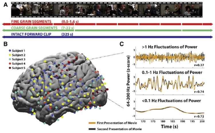
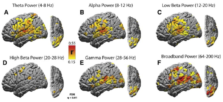
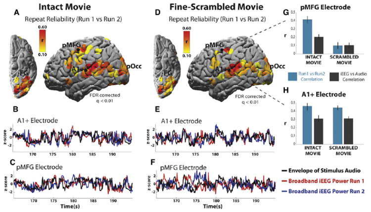
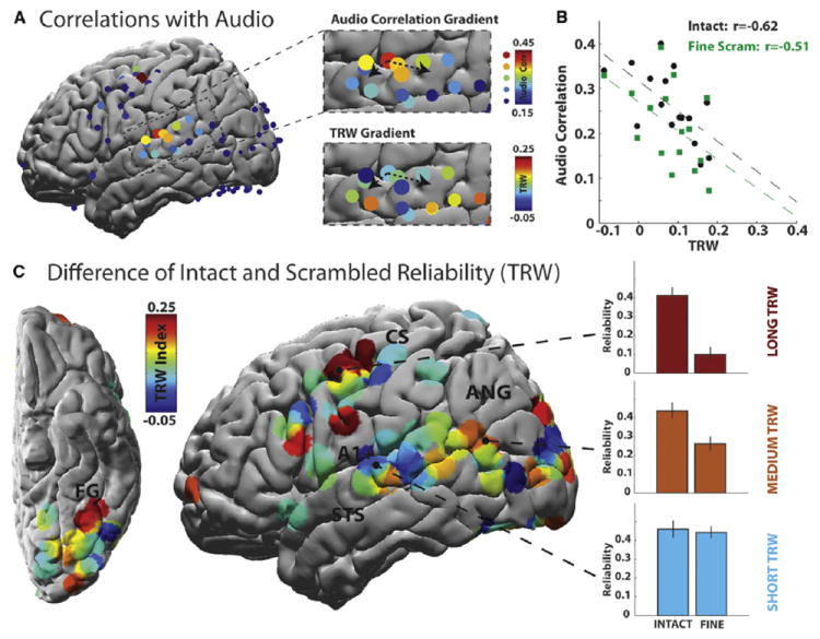
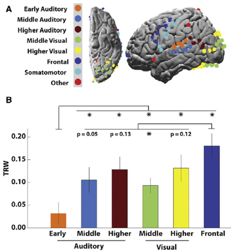
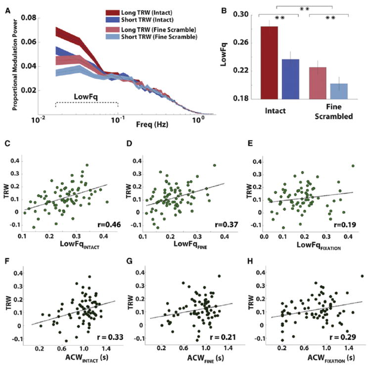
Making sense of the world requires us to process information over multiple timescales. We sought to identify brain regions that accumulate information over short and long timescales and to characterize the distinguishing features of their dynamics. We recorded electrocorticographic (ECoG) signals from individuals watching intact and scrambled movies. Within sensory regions, fluctuations of high-frequency (64-200 Hz) power reliably tracked instantaneous low-level properties of the intact and scrambled movies. Within higher order regions, the power fluctuations were more reliable for the intact movie than the scrambled movie, indicating that these regions accumulate information over relatively long time periods (several seconds or longer). Slow (<0.1 Hz) fluctuations of high-frequency power with time courses locked to the movies were observed throughout the cortex. Slow fluctuations were relatively larger in regions that accumulated information over longer time periods, suggesting a connection between slow neuronal population dynamics and temporally extended information processing.


Figures

Figure 1
Figure 1. Slow and Fast Responses to Intact and Scrambled Stimuli
(A) Illustration of the coherent segments used in the intact, coarse-scrambled and fine-scrambled movies. Movie stills are pixelated in this panel for copyright reasons. (B) Electrode coverage from five subjects, illustrated on an average MNI brain. Electrode colors indicate different subjects. (C) Example time courses from an early auditory region, illustrating the fast, medium and slow components of the single-trial neural response to a complex audiovisual stimulus. The responses to the first and second presentations are shown in yellow and gray, and Pearson correlation values across presentations are shown for each component.
Figure 2
Figure 2. Topography of Reliable Movie-Evoked Responses
(A) Reliability of 4–8 Hz θ power time courses across two presentations of the intact movie clip. (B) Reliability of 8–12 Hz α power time courses. (C) Reliability of 12–20 Hz low β power time courses. (D) Reliability of 20–28 Hz high β power time courses. (E) Reliability of 28–56 Hz γ power time courses. (F) Reliability of 64–200 Hz broadband power time courses. For each signal component, only electrodes reliable at the level q < 0.01 after FDR correction are shown. See also Figure S1.
Figure 3
Figure 3. Response Reliability and Relation to the Audio
(A) Reliability of responses across two presentations of the intact movie clip. Single-subject, single-electrode data is aggregated across five subjects on an MNI surface. (B and C) Single-electrode single-trial time courses of broadband power modulation in response to the first presentation (red curve) and second presentation (blue curve) of the stimulus, along with the time course of the audio envelope (black curve). (D–F) Reliability map and power time courses for the fine-scrambled movie clip, with same format as (A)–(C). (G and H) Bar plots show the correlation across stimulus repeats (blue bar), as well the correlation between ECoG power and the stimulus audio envelope (gray bar) for example electrodes in pMFG (G) and near primary auditory cortex (A1+, H). Electrodes that did not respond reliably to the intact movie are not shown. Error bars on the inset bar plots are SEM across 20 s sub-blocks. The same auditory electrode provides the example data for (B), (E), and (H); the same frontal electrode provides the example data for (C), (F), and (G). pMFG, posterior middle frontal gyrus; pOcc, posterior occipital cortex; FG, fusiform gyrus. See also Figure S5.
Figure 4
Figure 4. Topography of Stimulus Coupling and Temporal Receptive Windows
(A) Surface map showing correlation between neural responses and the amplitude of the stimulus audio. Top zoom inset: the audio correlation on the superior temporal gyrus; bottom zoom inset: TRW values on the superior temporal gyrus. The dotted arrows provide a visual reference for the proposed audio and TRW gradients. (B) TRW values of electrodes on superior temporal gyrus, plotted versus their correlation with stimulus audio in the intact condition (black circles) and fine-scrambled condition (green squares). For both intact and scrambled clips, regions with longer TRW show a weaker coupling to the audio envelope. (C) TRW topography aggregated across five individual subjects. Shorter TRWs are predominantly found nearer primary sensory areas, while longer TRWs predominate further away from sensory areas. The TRW index is defined as the difference in response reliability between the intact and scrambled stimuli. Error bars on bar plots indicate the SEM across 20 s sub-blocks of the data. STS, superior temporal sulcus; ANG, angular gyrus; CS, central sulcus. See also Figure S4.
Figure 5
Figure 5. ROI Analysis of TRW Differences
(A) Parcellation of reliable electrodes into ROIs. (B) Average TRW index within each ROI. We noted a progression of larger TRW indices for higher order cortical areas, with largest TRWs observed in frontal cortex. Error bars indicate SEM across electrodes within ROIs. *p < 0.05.
Figure 6
Figure 6. Intrinsic Slow Dynamics and the TRW
(A) Spectra showing the fraction of variance in the broadband fluctuations at frequencies between 0.01–1 Hz. Lines show the average of the normalized modulation spectra for two groups of electrode (long TRW in red and short TRW in blue) in two conditions (intact clip and fine-scrambled clip). Colored areas indicate SEM across 18 data samples, each 60 s. (B) The average amplitude of low-frequency fluctuations (LowFq, fraction of variance <0.1 Hz) for short TRW and long TRW electrodes. Error bars are SEM across electrodes. Asterisks indicate the significance of the comparison across electrode groups or conditions; *p < 0.05; **p < 0.01. The asterisk across the two pairs of bars indicates the aggregate difference across the intact and fine-scrambled conditions. (C–H) TRW of individual electrodes plotted versus their LowFq values in the intact movie (C) fine-scrambled movie (D) and fixation (E) conditions. (F–H) are for (C–E) with TRW plotted against ACW values. See also Figures S2–S6.
Figure 7
Figure 7. Fast and Slow Components of Response Reliability
(A) Average reliability across electrodes for all conditions. The reliability of power time courses (red bars) is increased after low-pass filtering at 0.1 Hz (gray bars) and decreased after high-pass filtering (blue bars), and this effect is strongest in the intact movie condition. Error bars indicate the SEM across electrodes. Asterisks indicate the significance of the comparison between low-pass and high-pass; *p < 0.05; **p < 0.01. (B) Reliability of individual electrodes to the intact stimulus versus their reliability in response to the fine-scrambled stimulus, with reliability computed after low-passing (gray dots) and high-passing (blue dots). The faster component of the power time course shows only a small difference in reliability between intact and scrambled movie, while the slow component shows a large difference. (C) Comparison of TRW values computed after low-pass and high-pass filtering plotted as a function of the original TRW values. Electrodes with large TRW values exhibited even larger TRW values after low-pass filtering. See also Figures S5 and S6.

References

    1. Ashburner J. A fast diffeomorphic image registration algorithm. NeuroImage. 2007;38:95–113. - PubMed
    1. Ben-Yakov A, Honey CJ, Lerner Y, Hasson U. Loss of reliable temporal structure in event-related averaging of naturalistic stimuli. Neuroimage. 2012;63:501–506. - PMC - PubMed
    1. Benjamini Y, Hochberg Y. Controlling the false discovery rate—a practical and powerful approach to multiple testing. J R Stat Soc Ser B. 1995;57:289–300.
    1. Bernacchia A, Seo H, Lee D, Wang XJ. A reservoir of time constants for memory traces in cortical neurons. Nat Neurosci. 2011;14:366–372. - PMC - PubMed
    1. Brody CD, Romo R, Kepecs A. Basic mechanisms for graded persistent activity: discrete attractors, continuous attractors, and dynamic representations. Curr Opin Neurobiol. 2003;13:204–211. - PubMed

Publication types

LinkOut - more resources