Spatially pooled contrast responses predict neural and perceptual similarity of naturalistic image categories

Abstract

The visual world is complex and continuously changing. Yet, our brain transforms patterns of light falling on our retina into a coherent percept within a few hundred milliseconds. Possibly, low-level neural responses already carry substantial information to facilitate rapid characterization of the visual input. Here, we computationally estimated low-level contrast responses to computer-generated naturalistic images, and tested whether spatial pooling of these responses could predict image similarity at the neural and behavioral level. Using EEG, we show that statistics derived from pooled responses explain a large amount of variance between single-image evoked potentials (ERPs) in individual subjects. Dissimilarity analysis on multi-electrode ERPs demonstrated that large differences between images in pooled response statistics are predictive of more dissimilar patterns of evoked activity, whereas images with little difference in statistics give rise to highly similar evoked activity patterns. In a separate behavioral experiment, images with large differences in statistics were judged as different categories, whereas images with little differences were confused. These findings suggest that statistics derived from low-level contrast responses can be extracted in early visual processing and can be relevant for rapid judgment of visual similarity. We compared our results with two other, well- known contrast statistics: Fourier power spectra and higher-order properties of contrast distributions (skewness and kurtosis). Interestingly, whereas these statistics allow for accurate image categorization, they do not predict ERP response patterns or behavioral categorization confusions. These converging computational, neural and behavioral results suggest that statistics of pooled contrast responses contain information that corresponds with perceived visual similarity in a rapid, low-level categorization task.

Figure 1. Contrast histograms of natural images follow a Weibull distribution.

(A), Three natural images with varying degrees of details and scene fragmentation. The homogenous, texture-like image of grass (upper row) contains many edges of various strengths; its contrast distribution approaches a Gaussian. The strongly segmented image of green leaves against a uniform background (bottom row) contains very few, strong edges that are highly coherent; its distribution approaches power law. Most natural images, however, have distributions in between (middle row). The degree to which images vary between these two extremes is reflected in the free parameters of a Weibull fit to the contrast histogram: β (beta) and γ (gamma). (B), For each of 200 natural scenes, the beta and gamma values were derived from fitting the Weibull distribution to their contrast histogram. Beta describes the width of the histogram: it varies with the distribution of local contrasts strengths. Gamma describes the shape of the histogram: it varies with the amount of scene clutter. Four representative pictures are shown in each corner of the parameter space. Images with a high degree of scene segmentation, e.g. a leaf on top of snow, are found in the lower left corner, whereas highly cluttered images are on the right. Images with more depth are located on the top, whereas flat images are found at the bottom. Images are from the McGill Calibrated Colour Image Database .

Figure 2. Example stimuli and computation of contrast statistics.

(A), Example images of each of the 16 categories used in the behavioral and EEG experiment. Images contained randomly placed disks that differed in distribution, opacity, depth and size. Each category contained 16 unique images. (B), Consecutive steps in computing various contrast statistics. Weibull statistics are computed by filtering the image with a range of contrast filters with LGN-like scale- and gain properties, after which for each image location, the filter containing the minimal reliable response is selected. Responses of all selected filters are summed in a histogram to which the Weibull function is fitted, from which the beta and gamma parameters are derived using maximum likelihood estimation. (C), Power spectra parameters (top row) are extracted by taking the Fourier transform, averaging across directions, and computing the intercept and slope values of a line fitted to the average power spectrum. Higher-order properties of the contrast distribution (bottom row) are computed by filtering with a single-scale center-surround filter, after which skewness and kurtosis of the resulting contrast distribution are derived. Weibull statistics (multiscale local contrast) presumably contain information present in Fourier parameters (scale statistics) as well as local contrast distribution parameters (distribution statistics).

Figure 3. Methods and experimental design.

(A), Experimental set-up of experiment 1 (EEG experiment). Subjects were presented with individual images of dead leaves while EEG was recorded. Single-image evoked responses (ERPs) were computed for each electrode, by averaging two repeated presentations of each individual image. Regression analyses of ERP amplitude on contrast statistics were performed at each time sample and electrode. (B), Representational dissimilarity matrices (RDMs) were computed at each sample of the ERP. A single RDM displays Euclidean distance (red = high, blue = low) between multiple-electrode patterns of ERP amplitude between all pairs of stimuli at a specific moment in time. The (cartoon) inset demonstrates how dissimilarities can cluster by category: all images from one category are in consecutive rows and can be ‘similarly dissimilar’ to other categories. (C), Experimental set-up of experiment 2 (behavioral experiment). On each trial, subjects were presented with a pair of stimuli for 50 ms, followed by a mask after an interval of 100 ms. Subjects were presented 8 times with all possible pairings of stimuli and were instructed to indicate whether stimuli were the same or different. (D), Cartoon example of leave-one-out classification based on contrast statistics. One stimulus is selected in turn, after which the median (thumbnail) of the remaining stimuli of its category is computed, as well as the median of other categories (here, just one). Classification accuracy reflects how many stimuli are closer to the median of other categories instead of its own category in terms of distance in image statistics.

Figure 4. Stimuli set out against their respective contrast statistics.

Each data-point reflects parameter values for a single image, color-coded by category. Individual images are displayed against their (A), Weibull parameters beta and gamma, (B), Fourier parameters intercept and (increasing negative) slope and (C), distribution properties skewness and kurtosis. In all cases, clustering by category based on parameter values is evident. (D), Non-parametric correlations between the six image parameters: Beta (B), Gamma (G), Fourier Intercept (Ic), Fourier Slope (S), Skewness (Sk) and Kurtosis (Ku).

Figure 5. Regression analysis of EEG data: single subject results.

Explained variance of ERP amplitude at channel Oz over time, for each individual subject (colored thin lines) and mean across subjects (black thick line), using as regressors either (A), Weibull parameters beta and gamma, (B), Fourier parameters intercept and slope and (C), skewness and kurtosis; single-trial results of these analyses can be found in Fig. S4. Insets display scalp plots of r² values for all electrodes at the time of maximal explained variance averaged over subjects (113 ms for Weibull/Fourier, 254 ms for skewness/kurtosis. (D), Grand average ERP amplitude (averaged over all subjects and all images) for an early and a late time-point of peak explained variance displayed in A–C.

Figure 6. AIC (Akaike information criterion) and unique explained variance analyses at channel Oz.

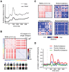
(A), Mean explained variance across single subjects for Weibull (red), Fourier (blue) and skewness/kurtosis (green), respectively; shaded areas indicate S.E.M. (B), Mean AIC-value across single subjects computed from the residuals of each of the three regression models, as well as an additional model (black) consisting of Fourier and skewness/kurtosis values combined, showing that Weibull parameters provide the best fit to the data (low AIC-value); shaded areas indicate S.E.M. (C), Single subject AIC-values for the models displayed in B at the time-point of maximal explained variance for Weibull and Fourier statistics (113 ms); subjects are sorted based on independently determined SNR ratio (reported in Fig. S2). (D), Unique explained variance by each set of contrast statistics. (E), Absolute, non-parametric correlations (Spearman's ρ) with ERP amplitude for the individual image parameters: Beta (B), Gamma (G), Fourier Intercept (Ic), Fourier Slope (S), distribution Skewness (Sk) and Kurtosis (Ku). Absolute values are plotted for convenience; shaded areas indicate S.E.M. (F), Unique explained variance by each individual parameter. Results for A–E based on single-trial rather than single-image data were highly similar (Fig. S5).

Figure 7. Results of RDM analysis.

(A), Maximum and mean Euclidean distance for the subject-averaged RDM: for both measures, highest dissimilarity between images was found at 101 ms after stimulus-onset. (B), Mean RDM across subjects at the moment of maximal Euclidean distance. Each cell of the matrix reflects the dissimilarity (red = high, blue = low) between two individual images, whose category is indexed on the x- and y-axis. (C), Dissimilarity matrices based on difference in contrast statistics between individual images. Color values indicate the summed difference between two individual images in beta and gamma (Weibull statistics), intercept and slope (Fourier statistics), skewness and kurtosis (distribution statistics). (D), Correlation between the RDM and each of the three dissimilarity matrices at each time-point. Highest correlation is found for Weibull statistics at 109 ms. Shaded areas reflect 95% confidence intervals obtained from a percentile bootstrap on the dissimilarity values.

Figure 8. Behavioral results and comparison with classification.

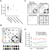
(A), Accuracy of behavioral categorization (open circles: single subjects, filled circle: mean) and of classification based on Weibull parameters, Fourier parameters or skewness and kurtosis. (B), Behavioral confusion matrix, displaying mean categorization accuracy for specific comparisons of categories. For each pair of categories the percentage of correct answers is displayed as a grayscale value. (C), Comparison of mean behavioral confusion matrix with classification results based on the three sets of contrast statistics. (D), Inter-matrix correlations of the classification errors for each set of statistics with the mean behavioral confusion matrix (left, mean) as well as those of individual participants (right, single subjects). For the mean correlation, error bars indicate 95% confidence intervals obtained using a percentile bootstrap on values within the mean confusion matrix.

References

1. Potter MC (1975) Meaning in visual search. Science 187: 965–966. - PubMed
1. Greene MR, Oliva A (2009) The briefest of glances: the time course of natural scene understanding. Psych Sci 20: 464–472. - PMC - PubMed
1. Fei-Fei L, VanRullen R, Koch C, Perona P (2002) Rapid natural scene categorization in the near absence of attention. Proc Natl Acad Sci U S A 99: 9596–9601. - PMC - PubMed
1. Thorpe S, Fize D, Marlot C (1996) Speed of processing in the human visual system. Nature 381: 520–522. - PubMed
1. Kirchner H, Thorpe SJ (2006) Ultra-rapid object detection with saccadic eye movements: visual processing speed revisited. Vision Res 46: 1762–1776. - PubMed
Publication types