A neural model for temporal order judgments and their active recalibration: a common mechanism for space and time?

Abstract

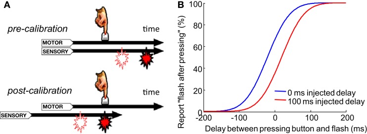
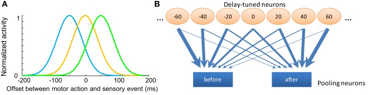
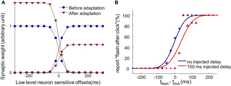
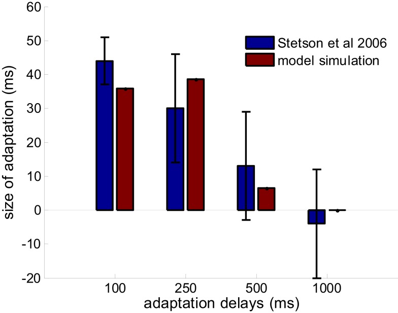
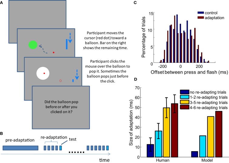
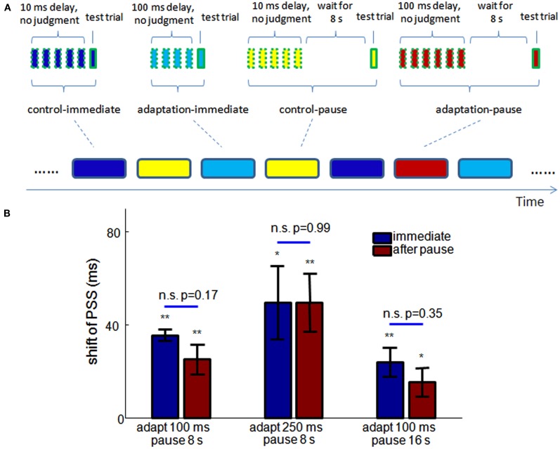
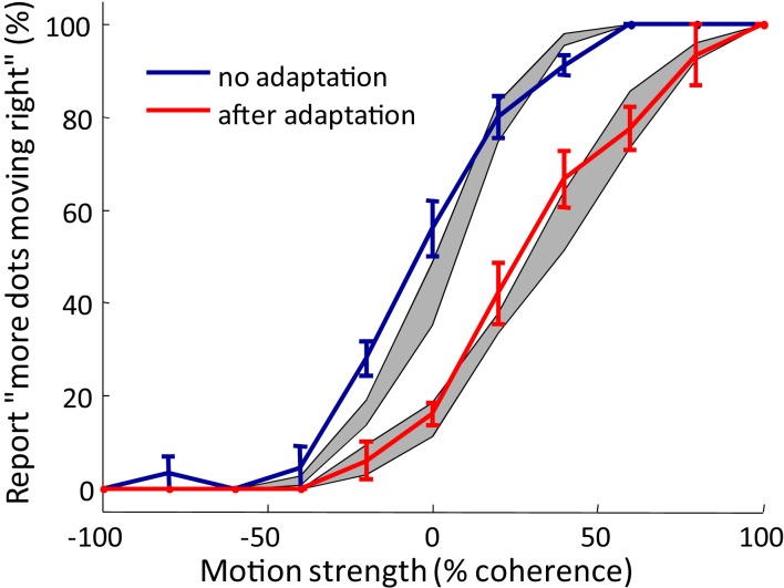
When observers experience a constant delay between their motor actions and sensory feedback, their perception of the temporal order between actions and sensations adapt (Stetson et al., 2006). We present here a novel neural model that can explain temporal order judgments (TOJs) and their recalibration. Our model employs three ubiquitous features of neural systems: (1) information pooling, (2) opponent processing, and (3) synaptic scaling. Specifically, the model proposes that different populations of neurons encode different delays between motor-sensory events, the outputs of these populations feed into rivaling neural populations (encoding "before" and "after"), and the activity difference between these populations determines the perceptual judgment. As a consequence of synaptic scaling of input weights, motor acts which are consistently followed by delayed sensory feedback will cause the network to recalibrate its point of subjective simultaneity. The structure of our model raises the possibility that recalibration of TOJs is a temporal analog to the motion aftereffect (MAE). In other words, identical neural mechanisms may be used to make perceptual determinations about both space and time. Our model captures behavioral recalibration results for different numbers of adapting trials and different adapting delays. In line with predictions of the model, we additionally demonstrate that temporal recalibration can last through time, in analogy to storage of the MAE.

Keywords: motion aftereffect; opponent processing; recalibration; synaptic scaling; temporal order judgment.

Figure 1

Recalibration of temporal order judgment after adapting to a constant delay between motion and sensory event. (A) A flash consistently appears with a fixed delay (filled icon) after a button press. If a flash is suddenly presented with a shorter delay (open icon), it will be perceived as appearing before the press after calibration. Stetson et al. (2006) proposed that this is due to the relative shift of the motor and sensory time lines (i.e., temporal expectations; reproduced from Stetson et al., , with permission; B). A cartoon of psychometric curves of a participant judging the temporal order between a button press and a flash. In the control condition, before each test trial, participants are presented with a flash immediately after each of 3–5 presses of the button. Then, in a testing trial, they report the perceived temporal order between their press and a flash that is randomly presented before or after the press. Data from the testing trials are plotted in blue. The red curve represents the adaptation condition, in which a constant 100 ms delay is injected between the flash and each of the 3–5 presses before the test trials. Curves based on average data from participants in Stetson et al. (2006).

Figure 2

Opponent processing model for temporal order judgments. (A) The tuning curves of several hypothetical “delay sensitive” neurons which have the strongest responses for specific delays between motor and sensory events. (B) Diagram of the pooling opponent processing circuits. Orange circles represent the hypothetic lower level delay sensitive neurons with different preferred delays between motor action and sensory input. Blue rectangles represent pooling modules with different input weight patterns from the lower level neurons; they selectively receive stronger synapses from neurons coding for “before” or “after,” respectively. The width of the arrows indicates the strength of the weights. These pooling modules compete with each other to reach a decision; the one with stronger activity will represent the final judgment of temporal order.

Figure 3

Synaptic scaling at the single neuron level in the pooling populations gives rise to recalibration. (A) Illustration of the change to the weights of the pooling modules (the one-directional arrows pointing to the blue rectangles in Figure 2B) after the system is constantly exposed to a 100 ms delay between an action and a sensory event. Before adaptation, the weights of the pooling modules are balanced, as shown by the blue circles. After adapting to a constant positive delay, the pooling populations encoding for “flash after press” globally decreases their weights and the pooling populations encoding for “flash before press” globally increase their weight, as shown by the red triangles. (B) The psychometric curve obtained by simulating the network proposed in Figure 2B. The psychometric curve shifts so that a delayed sensory event is perceived simultaneously with the motor action. The finite slope of the curve comes from the Poisson-like noise on the lower level neurons and the gradual scaling of synaptic weights after a constant injected delay.

Figure 4

Prediction of the model on the limited adaptation size for large adaptation delay (red bars). Results from Stetson et al., are reproduced in blue bars with permission (n = 25, 5, 4, 4 for the adapting delays of 100, 250, 500, and 1000 ms). The delay-tuned neurons have a limit on the offsets that they can encode, which gives rise to this limited capacity of recalibration.

Figure 5

The size of adaptation increases as participants are exposed to more re-adapting trials before each test trial, as predicted by the model. (A) Task of the experiment: participants control the red dot with the mouse, and hit the static green disc representing a balloon. A shrinking blue bar on the right indicates the time left for popping the balloon. In adapting trials, if the participant presses before the time bar shrinks to bottom, the balloon pops (color change to white) with constant delay after the press. In test trials it pops before or after the press is made. Participants only need to judge the order of click and flash for test trials. In the real experiment, the dashed arrows are not seen. (B) Structure of an experiment block: 50 pre-adaptation trials lead to testing phase, in which each test trial is preceded by a random number of re-adapting trials (no such re-adapting trial in 0 re-adapting trial condition). (C) The distribution of the temporal offset for test trials is well balanced in both the control and adaptation blocks. The figure shows the distribution in the 3–5 adapting trial condition across all participants. (D) Using the parameter set obtained in Limited recalibration with increased adapting delays, the model successfully captures the average result of behavioral data. Error bars = SEM. n = 31, 16, 18, 15.

Figure 6

Storage of TOJ recalibration. (A) Experimental design. Meta-trials of four different conditions (indicated by the round-corner rectangles at the bottom) are randomly interleaved in the experiment. Each meta-trial consists of 4–6 adapting trials (squares of dashed outline) and one test trial, with additional 8 s wait time in the control-pause and adaptation-pause conditions (the pause is 16 s in the third experiment). (B) The shifts of PSS from control to adaptation conditions in the three experiments (n = 10, 10, 9). No significant difference of the shifts of PSS is observed with and without a pause before a test trial, in any of the experiments. Blue: test trial immediately follows adapting trials. Red: a pause is inserted between adapting trials and the test trials. *significantly different from 0, p < 0.05, **p < 0.01. Errorbar: SEM.

Figure 7

Typical psychometric curves showing motion aftereffect, as tested with random dot kinematograms. Solid lines: psychometric curves averaged over participants (n = 5). Error bar = SEM Red curve: adaptation condition in which participants view 15 s of dots moving rightward before each test stimulus of varying coherence that lasts 0.5 s. Blue curve: control condition in which there is no adapting stimulus preceding the test stimulus. Grey areas: simulation result from the model in Relation of the model to motion direction judgments (mean ± SEM). Repeat = 5.

References

-
- Albright T. D. (1984). Direction and orientation selectivity of neurons in visual area MT of the macaque. J. Neurophysiol. 52, 1106–1130 - PubMed
- Anstis S. M. (1975). “What does visual perception tell us about visual coding,” in Handbook of Psychobiology, eds. Gazzaniga M., Blakemore C. B. (New York, NY: Academic Press; ), 269–323
Grants and funding
LinkOut - more resources
Full Text Sources
Research Materials