Developmental origin of patchy axonal connectivity in the neocortex: a computational model

Abstract

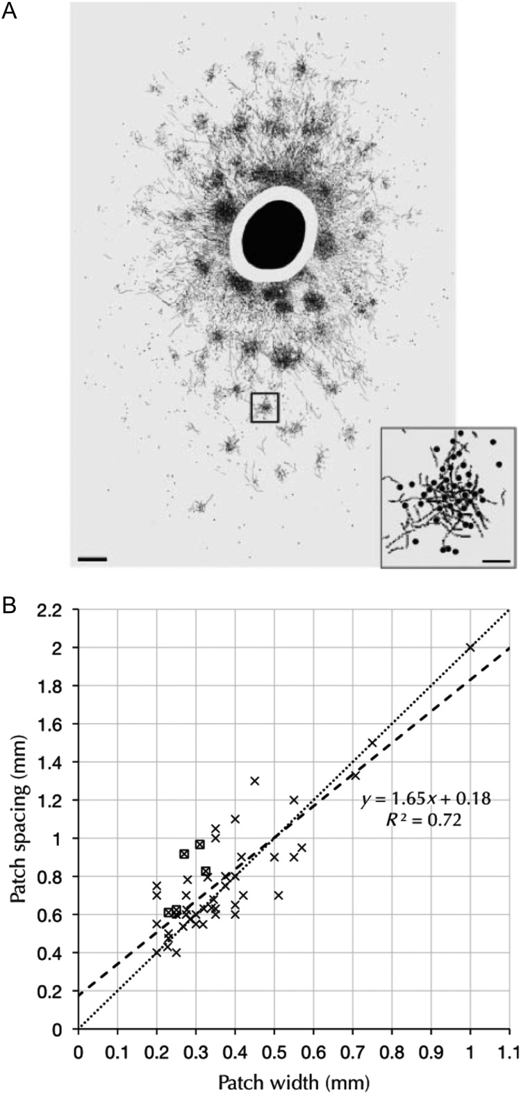
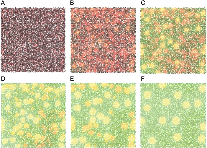
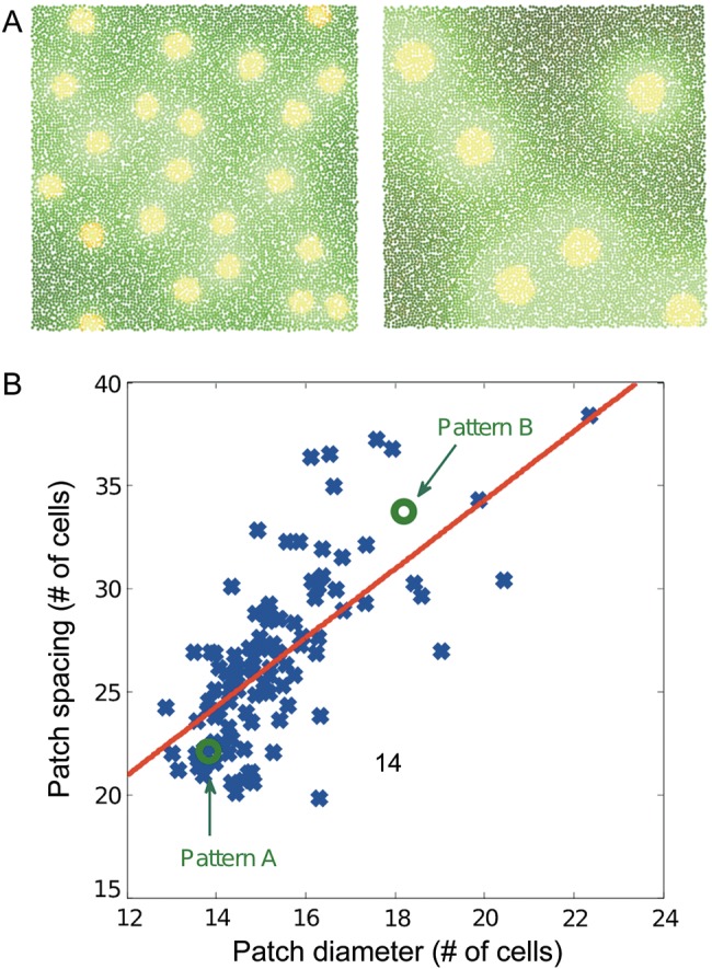
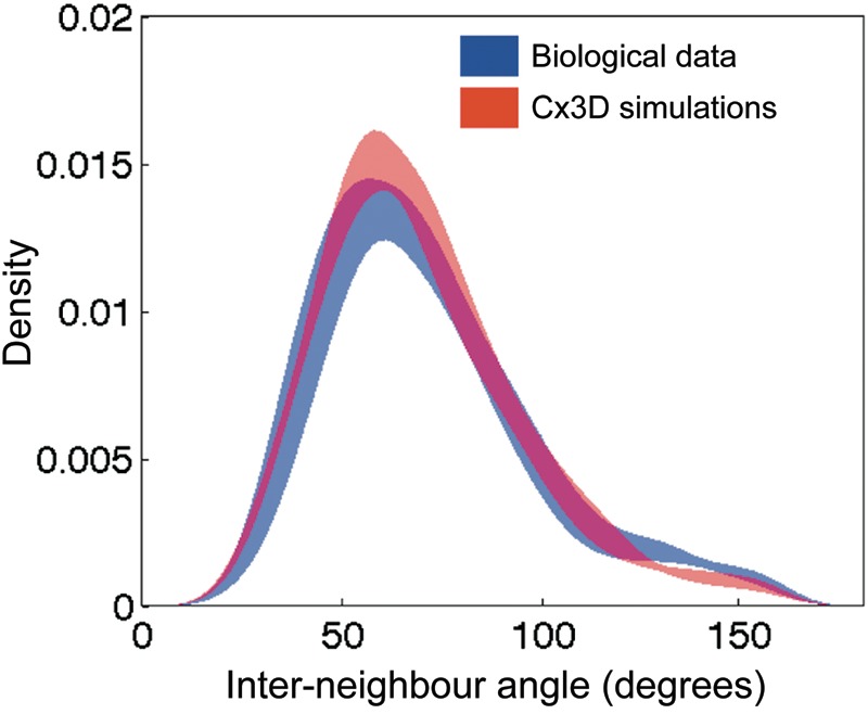
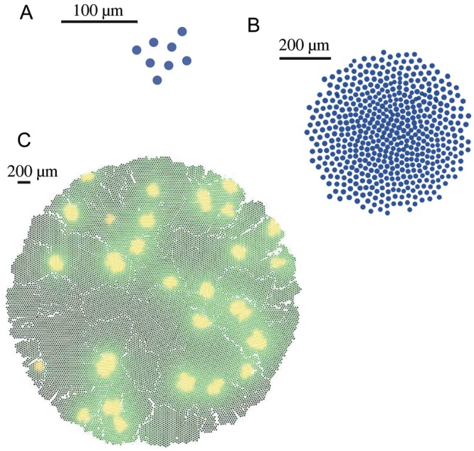
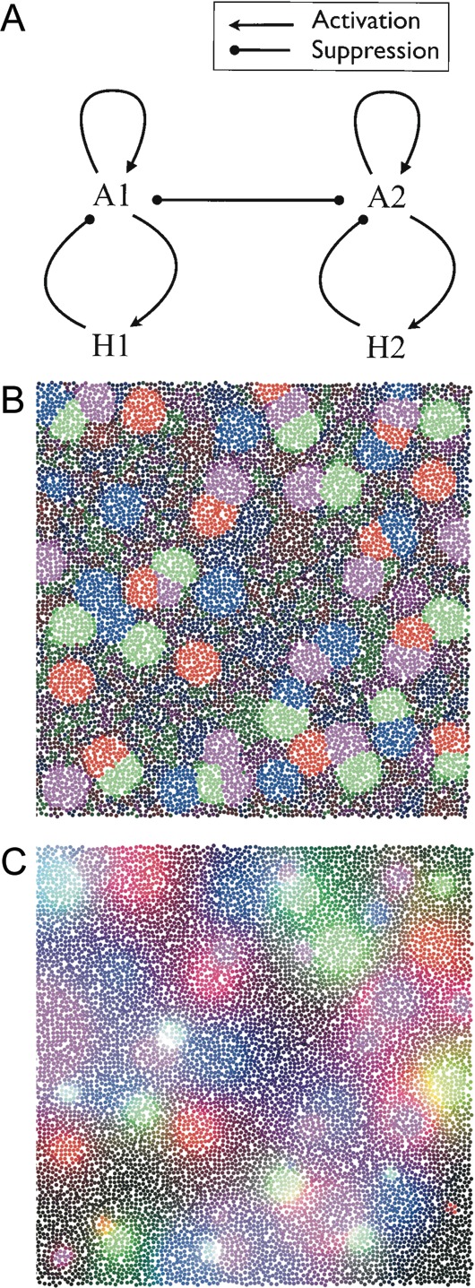
Injections of neural tracers into many mammalian neocortical areas reveal a common patchy motif of clustered axonal projections. We studied in simulation a mathematical model for neuronal development in order to investigate how this patchy connectivity could arise in layer II/III of the neocortex. In our model, individual neurons of this layer expressed the activator-inhibitor components of a Gierer-Meinhardt reaction-diffusion system. The resultant steady-state reaction-diffusion pattern across the neuronal population was approximately hexagonal. Growth cones at the tips of extending axons used the various morphogens secreted by intrapatch neurons as guidance cues to direct their growth and invoke axonal arborization, so yielding a patchy distribution of arborization across the entire layer II/III. We found that adjustment of a single parameter yields the intriguing linear relationship between average patch diameter and interpatch spacing that has been observed experimentally over many cortical areas and species. We conclude that a simple Gierer-Meinhardt system expressed by the neurons of the developing neocortex is sufficient to explain the patterns of clustered connectivity observed experimentally.

Keywords: neural development; reaction–diffusion models; self-organization; simulation; superficial patch system.

Figure 1.

(A) Patchy labeling of somata and terminals in layer II/III in the macaque visual cortex following bulk injection of the tracer cholear toxin B subunit (from Lund et al. 2003, with permission). (B) Scaling of interpatch distance with patch diameter observed across various cortical areas and species (from Muir et al. 2011, with permission).

Figure 2.

Sequence of images from a Cx3D simulation showing the development of a Gierer–Meinhardt pattern over time. The neuronal cell bodies (somata) are colored spheres. Black indicates low morphogen concentration near the cell body. Red and green indicate the presence of high levels of activator and inhibitor substance concentrations, respectively (in the yellow patches, both morphogens are strongly concentrated). Initially, the morphogen concentrations and the locations of cell bodies are randomized over the 2-dimensional plane (A). The overabundance of patches at the earlier stages of pattern formation converges, by mutual competition, to a stable pattern of fewer and more separated morphogen concentration peaks (B–F).

Figure 3.

(A) Two Gierer–Meinhardt patterns generated in Cx3D having different characteristic patch diameters and interpatch distances. The only difference between the 2 cases is the production coefficient: ρ = 600 for the left pattern and ρ = 35 for the right pattern. (B) Influence of the production coefficient ρ on the patch size and interpatch spacing. Each sample point (blue) indicates a separate simulation with different ρ. Average patch diameters and interpatch distances are linearly related. The equation of the fitted linear interpolation (red) is y = 1.72 x + 0.15 (R² = 0.46, P-value <1 × 10⁻⁴), approximating closely the slope of 1.65 obtained from the experimental data (Muir et al. 2011). Note the increased density of sampling points toward the lower left, which has also been observed in biological systems.

Figure 4.

Comparison of the probability density functions of the measured interpatch angles from experimental data of the cat and macaque monkey (blue) and Cx3D simulations (red). Shading corresponds to the 90% confidence interval, as estimated by bootstrap analysis. The distributions are not different according to a 2-sample Kolmogorov–Smirnov test at the 5% significance level.

Figure 5.

Self-organized development of a patchy pattern. The initial precursor cell divides in the 2D plane, giving rise to several daughter cells (A: early division phase, B: progressed division phase). Cell division continues until an intracellular concentration reaches a predefined threshold, which stops the cell division. Based on this preplate, the Gierer–Meinhardt reaction–diffusion mechanism leads to a patchy pattern (C). A video of the self-organization of multiple patchy patterns is included in Supplementary Material (Supplementary Movie 5).

Figure 6.

(A) Interactions of 2 Gierer–Meinhardt systems. In addition to the basic antagonism of the activator and inhibitor morphogens (as used in the single-patch system scenario), the activator substances of different Gierer–Meinhardt systems inhibit each other. Sufficiently strong inhibition between different activator morphogens ensures that patches belonging to distinct systems do not overlap. (B) Simulation of 4 interacting patch systems from a Cx3D simulation. Each system is based on 2 morphogens interacting according to the Gierer–Meinhardt model. Red, green, blue, and purple indicate the concentrations of distinct activator substances. Repulsion constants between activators were chosen to be identical for all of the activator pairs. (C) Multiple patch systems defined by inhibitory substances (same simulation as in Fig. 6B). Red, green, blue, and purple indicate the concentrations of distinct inhibitor types. In contrast to the scenario where patches are defined by the activator substance concentration, here, there is a smooth overlap between patches because there is no mutual inhibition between inhibitory substances. Patch systems are still guaranteed to develop at distinct locations, because the different activator substances compete with each other, such that also the patches of the inhibitor concentrations are at different locations.

Figure 7.

(A and B) Effect of variation in the production efficacy on patch locations. (A) Superimposition of the activator morphogen concentrations (red and blue label the 2 activator types) of 2 different noninteracting Gierer–Meinhardt systems. There is no variation, and the repulsion constant between the 2 activators is set to 0. Therefore, patches of both systems emerge at random and independent locations. For clearer visualization, overlapping patches are indicated with white circles. (B) Obtained when there was a nonzero variance on both the cellular production coefficient ρ and the basal production coefficients ρ_a and ρ_h (equations 1). The variance allows some patchy organizations to be preferred over others, because those patches will fall predominantly onto the same highly productive locations. High concentrations of both activator types are colored purple, because red and blue are added. (C and D) The magnitude of the repulsion coefficients determines the distance of the different patch systems. (C) Two superimposed concentration patterns of the activator morphogens from interacting Gierer–Meinhardt systems with small repulsion coefficients. In addition, production coefficients across the cells vary in a Gaussian manner. Due to the low repulsion, the patches of the 2 systems end up quite close to each other. (D) Two interacting Gierer–Meinhardt systems with strong repulsion. The patches of the different patch systems repel another more from the preferred locations than in (C). This was confirmed by calculating the average distances between patches belonging to distinct patch systems.

Figure 8.

Daisy architecture in a laminated cortical structure. Multiple patch systems (A: diagonal top-down view, B: straight top-down view) generated from an initial 2D sheet, which is the cortical plate before lamination of the cortex. Information that establishes which system a cell belongs to is preserved in the vertical direction. Red, green, blue, and purple indicate cells that belong to the 4 different patch systems. Supragranular layers are labeled gray, infragranular are black. Cells labeled as belonging to a patch system, and located in layer II/III, continue producing the activator substance that is used by the axonal growth cones to establish the long-range connectivity, as shown in Figure 9B. The simulation consists of 100 × 100 cells in a slab 18 cells thick.

Figure 9.

(A) Development of axonal long-range projections on a single-patch system. Growth cones of randomly selected cells follow the gradient of an extracellular cue secreted by cells located inside the patches. This same cue promotes more dense arborization by increasing the probability of the axon to bifurcate. (1) Initially, cells extend their axons in random directions. The yellowish somata are the strongest producers of the guidance cue. Newly extended axons and their cell bodies are colored red. (2 and 3) The region of high guidance cue concentration (yellow cell bodies) already has denser arborizations. (4) Arborization pattern at progressed stage. For the sake of clearer visualization, we set the bifurcation probability outside the patches to be quite low. (B) Sequence of axonal growth on multiple patch systems from the pattern in Figure 6B. This axonal growth rule makes use of many patchy patterns generated by the Gierer–Meinhardt model. In contrast to the simpler growth rule with only 1 global patch system, in this case, the location of the soma determines the targeted activator type (different colors indicate different types). Axons that arise from cell bodies lying in a patch will make long-range projections only to the patches of a similar identity. Cell bodies that are not located inside a region of high activator and inhibitor concentration levels make only nonspecific local connections. The specificity of the resulting connections can be controlled by the parameters of the growth model. For example, as mentioned in the Materials and Methods section, the probability to bifurcate is given by , where is the concentration of the activator substance and u, v are variable parameters. Large v increases the probability to branch outside of the patches, leading to less specific connectivity. In the scenario with multiple patch systems, a growth cone could also target activator patches of multiple types with different scaling parameters u, such that the communication between different patch systems is increased. Additionally, the bifurcation could be guided by the inhibitor substance, which increases the overlap between different patch systems (as shown in Fig. 6B,C).

References

1. Angelucci A, Sainsbury K. Contribution of feedforward thalamic afferents and corticogeniculate feedback to the spatial summation area of macaque V1 and LGN. J Comp Neurol. 2006;498:330–351. - PubMed
1. Binzegger T, Douglas R, Martin K. Stereotypical bouton clustering of individual neurons in cat primary visual cortex. J Neurosci. 2007;27:12242–12254. - PMC - PubMed
1. Binzegger T, Douglas R, Martin K. An axonal perspective on cortical circuits. In: Feldmeyer D, Lübke JHR, editors. New aspects of axonal structure and function. New York (NY): Springer; 2010. pp. 117–139.
1. Bonabeau E. From classical models of morphogenesis to agent-based models of pattern formation. Artif Life. 1997;3:191–211. - PubMed
1. Bosking W, Zhang Y, Schofield B, Fitzpatrick D. Orientation selectivity and the arrangement of horizontal connections in tree shrew striate cortex. J Neurosci. 1997;17:2112–2127. - PMC - PubMed
Publication types