

Review
doi: 10.1021/cr3002142.
Epub 2012 Nov 12.
Beyond gel electrophoresis: microfluidic separations, fluorescence burst analysis, and DNA stretching
Affiliations
- PMID: 23140825
- PMCID: PMC3595390
- DOI: 10.1021/cr3002142
Item in Clipboard
Review
Beyond gel electrophoresis: microfluidic separations, fluorescence burst analysis, and DNA stretching
Chem Rev.
.
No abstract available
Figures
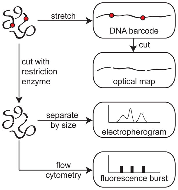
Schematic illustration of different approaches to obtain genomic information. The typical resolution of these methods is 1 kilobase pair (kbp). The red dots are meant to depict the location of restriction sites (when the DNA is cut at these location) or the location of some probe molecule (for DNA barcoding).
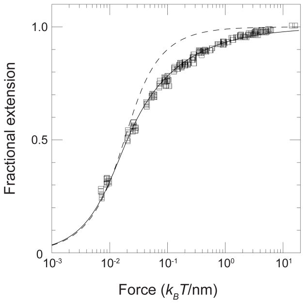
Fit of the wormlike chain model to the experimental force-extension behavior for a 97 kbp DNA. The solid symbols are experimental data. The solid line is the numerical solution of the wormlike chain model using a persistence length of lp = 53 nm and a contour length L = 32.8 μm. The dashed curve is the prediction of a freely jointed model with a segment length b = 100 nm. Reprinted with permission from Ref. Copyright 1995 American Chemical Society.
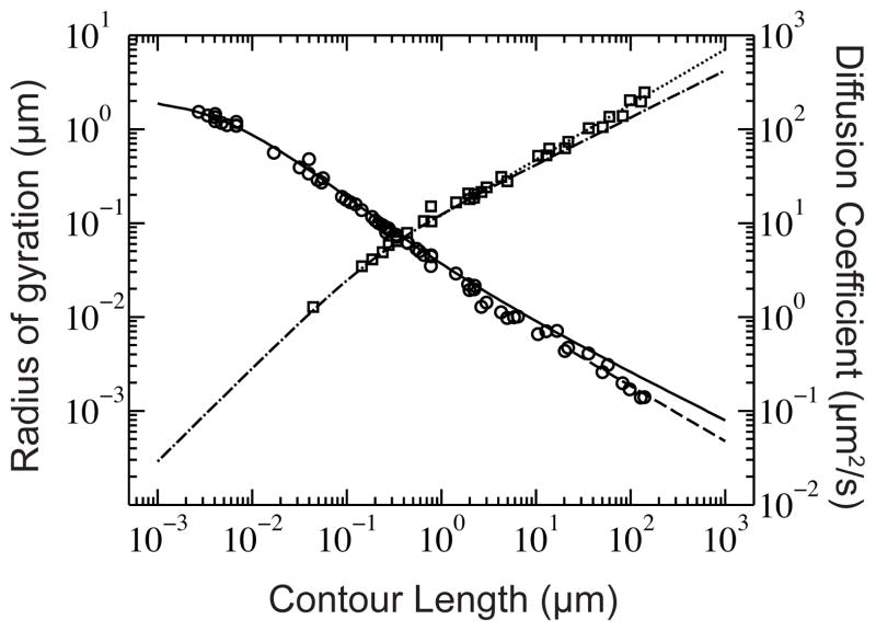
Radius of gyration (squares) and diffusion coefficient (circles) of DNA for a wide range of experimental conditions found in literature.– The solid line represents the diffusion coefficient of a wormlike chain, according to the theory of Yamakawa with a bead hydrodynamic radius of 1.14 nm; the dashed line indicates diffusive scaling like N−ν. The dash-dot line is Eq. (2) and the dotted line shows the Nν scaling for the radius of gyration. Table S1 lists of each experimental data point and the corresponding value of the ionic strength. As we will discuss in Section 2.2, the different ionic strengths change the persistence length of the DNA, which can be a source of the scatter in the data.
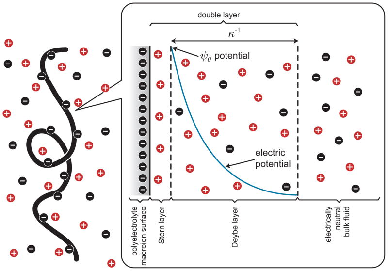
Schematic illustration of the local electrostatics near a DNA coil in free solution.
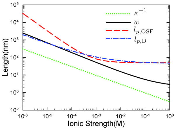
Calculation of the Debye length, effective width, and persistence length as a function of ionic strength using two different models for the persistence length. The persistence length lp;OSF is computed from the Odijk-Skolnick-Fixman theory in Eq. (12) and alternate value, lp,D, is computed using the theory from Dobrynin in Eq. (13). The effective width, w, is obtained from Stigter’s theory., Adapted with permission from Ref. Copyright 2008 American Chemical Society.
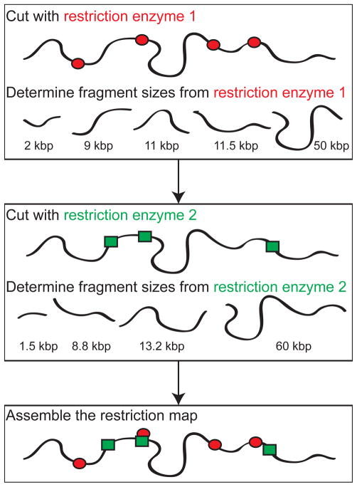
Schematic illustration of restriction mapping. Typical restriction maps of genomes include the locations of numerous restriction sites; the map produced by the example shown here would only correspond to two restriction enzymes (the red ellipses and green rectangles) with seven total restriction sites.
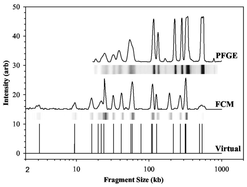
Comparison of pulsed field gel electrophoresis (PFGE) electropherograms and flow cytometry (FCM) for SmaI digested S. aureus Mu50. The raw PFGE data are the bands, which have been converted into a set of peaks, and the raw FCM data are the peaks, which have been converted into bands. The virtual digest is the expected location of the peaks based on the sequence of this strain. Reprinted with permission from Ref. Copyright 2004 American Society for Microbiology.
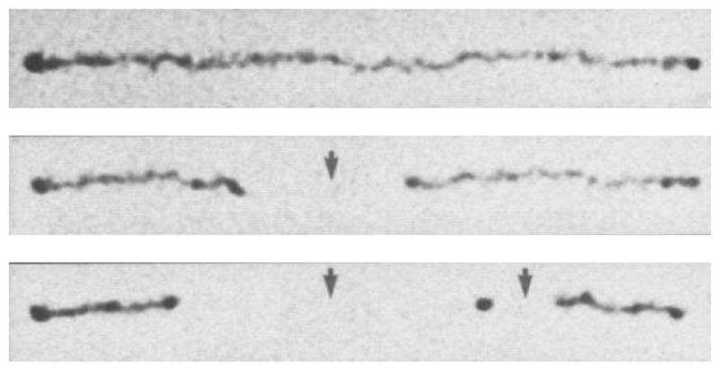
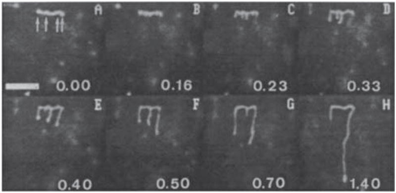
Time elapsed fluorescence micrograph of a stretched DNA molecule in molten agarose (image color inverted from the original). The arrows mark sites for CspI restriction endonuclease cleavage. Adapted with permission from Ref. Copyright 1993 American Association for the Advancement of Science.
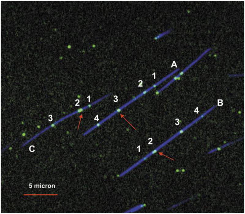
DNA barcoding using nicking enzymes and fluorescent nucleotides. The blue color corresponds to a YOYO labeled backbone and the green color corresponds to nicking enzyme sites. Each labeled fragment (A, B, and C) contains seven nicking sites, but only four (numbered 1–4) are distinguishable — due to diffraction — on molecules A and B and only three are distinguishable on fragment C. Red arrows indicate clustered nicking labels (for 2 which has three nicking sites and for 3 which has two). Adapted with permission from Ref. Copyright 2007 Oxford University Press.
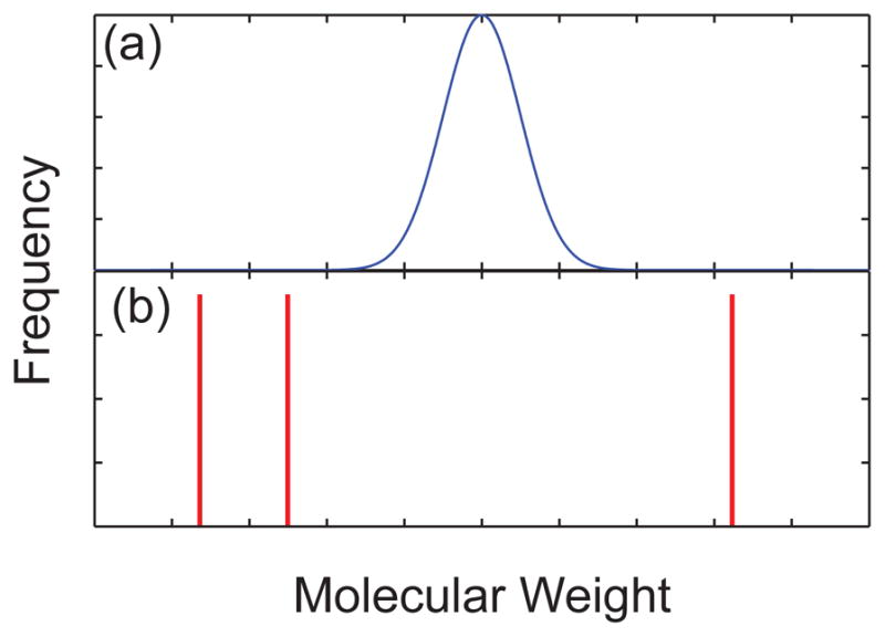
Schematic illustration of the molecular weight distribution for (a) a synthetic polymer and (b) a mixture of different sized DNA.
Schematic illustration of the difference between (a) the microscopic details of DNA migration in a microfabricated separation device and (b) the macroscopic viewpoint used to analyze the separation. The microchannel in (b) contains many obstacles, and the schematic shows two different sized DNA that have been separated due to their different migration speeds through the matrix. Note the different length scales in (a) and (b).
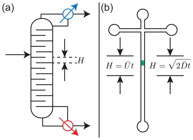
(a) Standard definition of a theoretical plate in distillation, an example of an equilibrium-based separation process. (b) Extension of the concept of theoretical plate heights in the context of a non-equilibrium separation. In a separation, the theoretical plate height H is a mathematical definition and not associated with a physical region of the device or the location of the band.
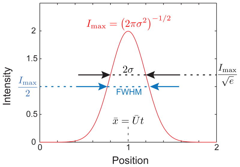
Snapshot of a Gaussian function with unit mass, Ū = 0.5, and D̄ = 0.01 at time τ = 2. The maximum value of the intensity, Imax, the variance in intensity, σ, the full width half maximum (FWHM), and the location of the maximum value of the intensity, x = Ūt, are indicated.
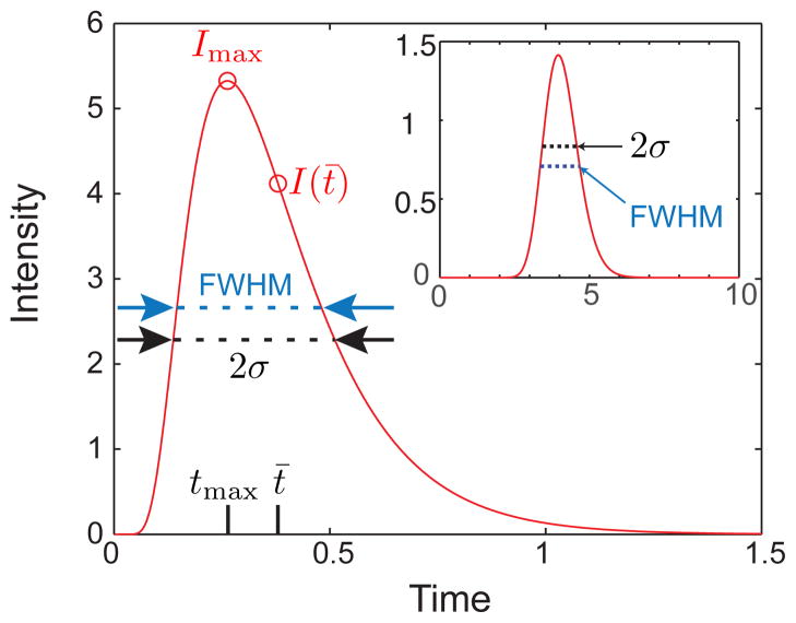
Finish line detection of a Gaussian function with unit mass, Ū = 0.5, and D̄ = 0.01 at position L = 0.15. The velocity and dispersion coefficient are identical to Figure 13. The maximum value of the concentration, Imax, the variance, σ, the full width half maximum (FWHM), and the location of the concentration at the mean elution time, I(t̄), are indicated. The inset shows the same Gaussian peak measured at L = 2.
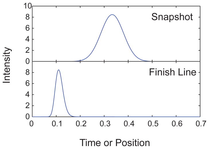
Comparison of the snapshot and finish line detection of a Gaussian function with unit mass, Ū = 3, and D̄ = 0.01 for Pe = 100. The choice of Péclet number fixes the equivalence between the length of the separation for the finish line, L = Pe(D/U), and thus the residence time, tr = L/U, for the snapshot detection.
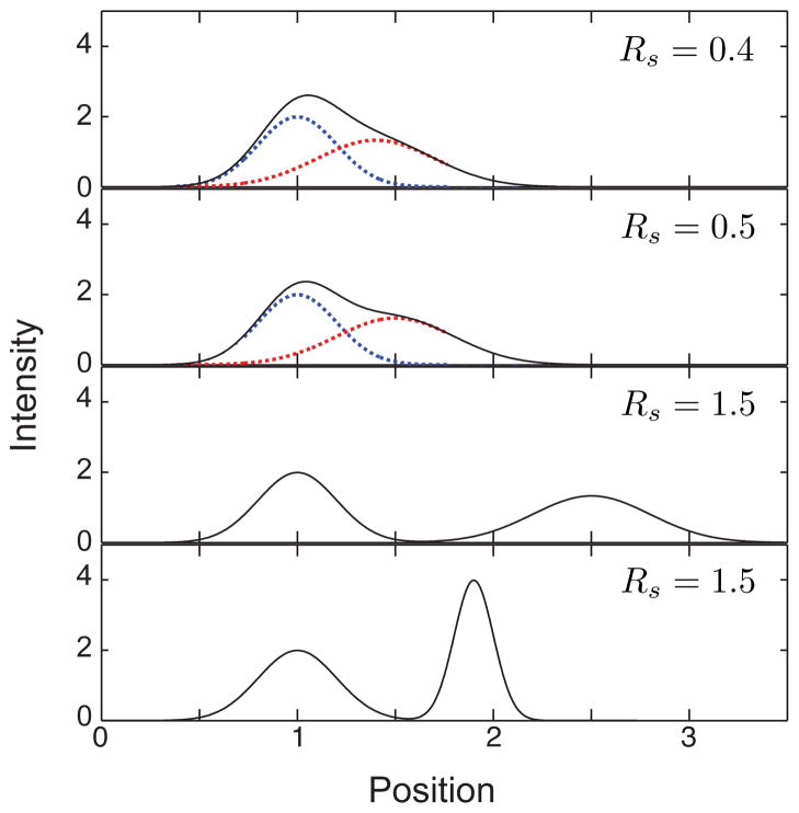
Illustration of different values of the resolution, Rs, for the case ξ = x. The solid black line corresponds to the total intensity at the detector. The dashed blue lines correspond to a peak with x̄ = 1 and σ = 0.3. The dashed red lines correspond to a second peak that produces the desired resolution. In the top three panels, the red curve has σ = 0.3. In the bottom panel, the red curve has σ = 0.1. Since the peaks are base line resolved for Rs = 1.5, only to the total intensity is shown.
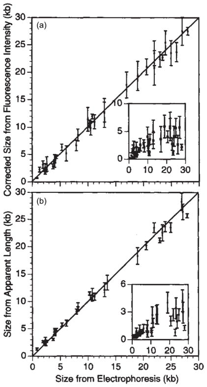
Calibration of (a) integrated fluorescence intensity and (b) apparent extension, which are measures of the chain size versus size measured from electrophoresis. The insets are estimations of the standard deviations of the population. Adapted with permission from Ref. Copyright 1995 Nature Publishing Group.
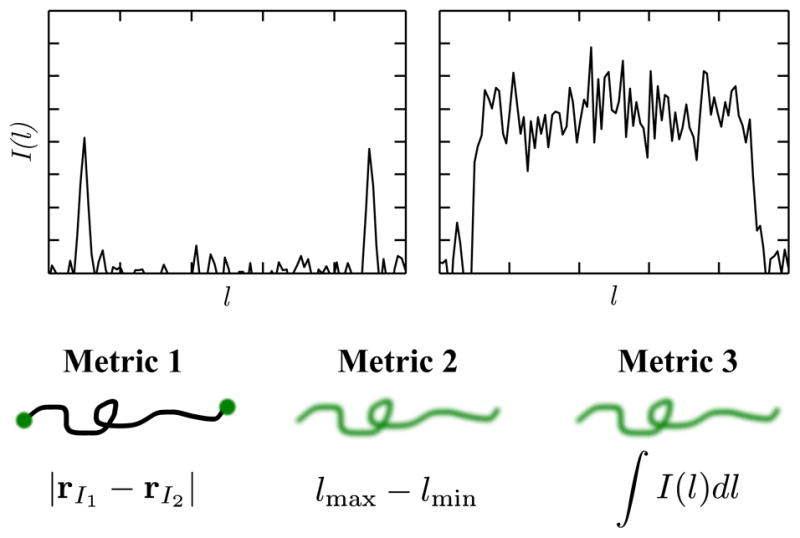
Three different methods to obtain a measure of genomic length using fluorescence microscopy: (1) Probe-probe distance, (2) extension, (3) integrated intensity. Plots show simulated fluorescence profiles for probes (left) and for intercalating dyes (right). The area under the curve on the right gives the total fluorescence intensity.
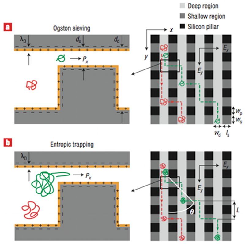
Schematic illustration of Ogston sieving. The DNA is small compared to the pore size in the gel so it can move freely through the interstices without deformation. Note that the pore spacing in the “gels” in Figure 20 and Figure 21 is identical to this figure, but the DNA is longer.
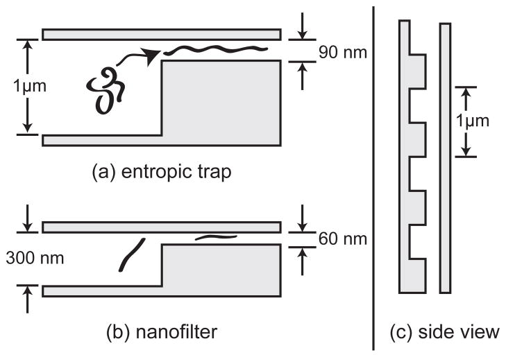
Schematic illustration of entropic trapping. Some of the pores are large enough for the DNA to fit inside without any deformation. To move between the trapping sites, the DNA needs to deform from its equilibrium coil to squeeze through the narrower constrictions. The dashed lines show the volume occupied by the DNA.
Schematic illustration of biased reptation. The chain is confined by the fibers of the gel to a reptation tube (dashed, red line). The arrows indicate possible directions for the chain to move along the tube. In the biased reptation model, the probability of moving in one of these two directions is biased by the electric field. A key assumption in the reptation theory is that the chain is confined inside the tube and cannot form hernias.
Schematic of (a) an inhomogeneous pulsed field setup with φ = 90° and (b) a homogeneous φ =120° (hexagonal) CHEF configuration.
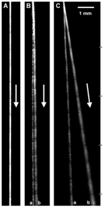
Reorientation of T2 DNA during pulsed field gel electrophoresis. Image (A) was taken a few seconds after the electric field in the horizontal direction was turned off and immediately before the electric field of 20 V/cm in the vertical direction was turned on. The scale bar is 8 μm. Reprinted with permission from Ref. Copyright 1990 American Chemical Society.
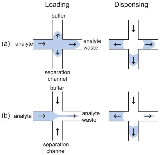
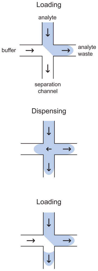
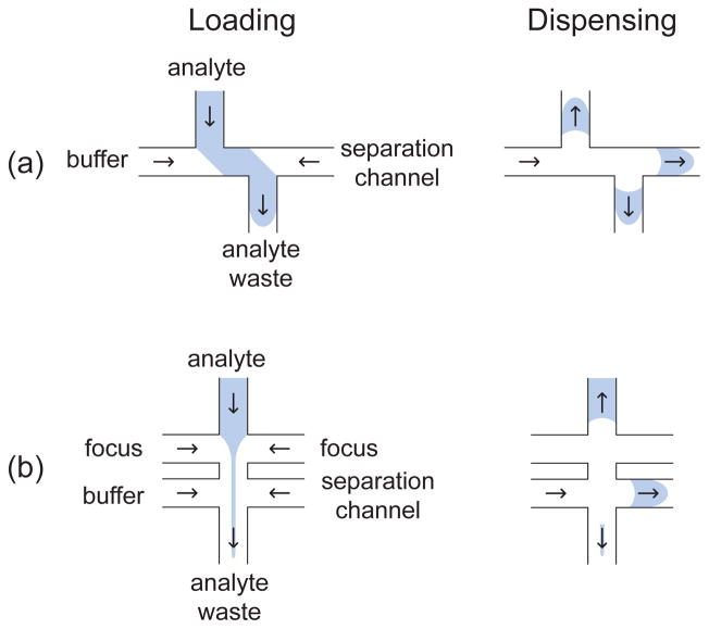
Injection and dispensing steps for (a) a floating injection and (b) a pinched injection. The arrows indicate the direction of the analyte transport in the different channels. For the case of a negatively charged species such as DNA, the arrows correspond to the direction opposite to the electric field.
Loading, dispensing, and reloading of a gated injection. The arrows indicate the direction of the analyte transport in the different channels. For the case of a negatively charged species such as DNA, the arrows correspond to the direction opposite to the electric field.
Loading and dispensing steps for (a) double-T and (b) multi-cross injections. The arrows indicate the direction of the analyte transport in the different channels. For the case of a negatively charged species such as DNA, the arrows correspond to the direction opposite to the electric field.
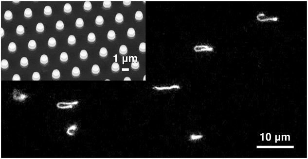
Epifluorescence microscopy image of dyed λ DNA molecules interacting with a hexagonal array of 1 μm diameter oxidized silicon posts. The electrophoretic motion at 10 V/cm is from left-to-right. The inset shows an SEM image of the oxidized post array. This previously unpublished figure was produced in the course of the research leading to Ref. The details of the experimental system are described in the latter reference.
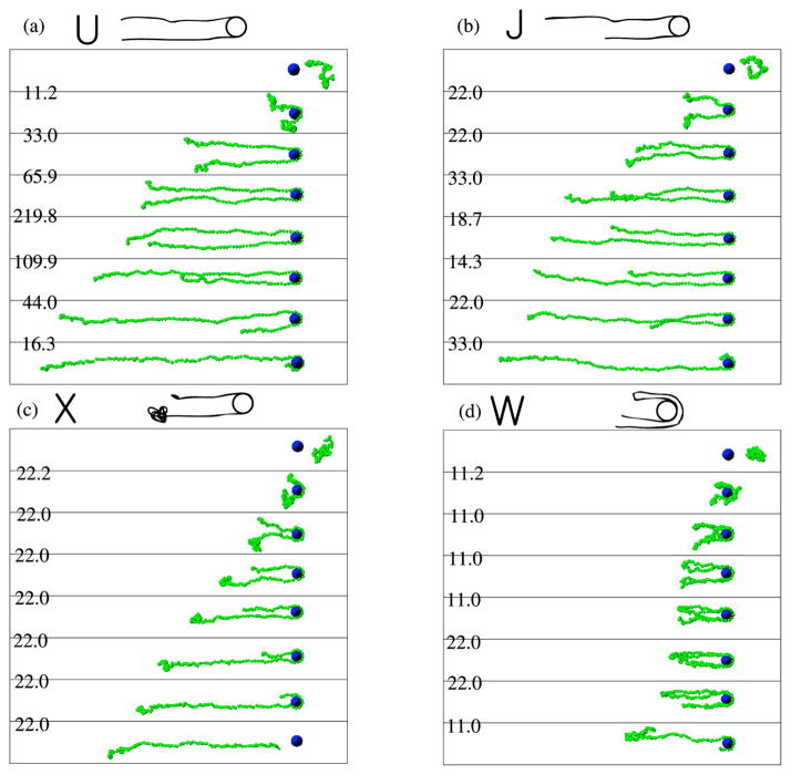
Examples of (a) U, (b) J, (c) X, (d) W collisions of T4-DNA (166 kbp) with an isolated 1.6 μm diameter post during Brownian dynamics simulations. The numbers on the left side of the images correspond to the dimensionless time between two successive snapshots. Reprinted with permission from Ref. Copyright 2007 American Chemical Society.
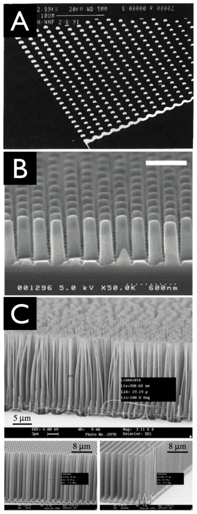
SEM images of microfabricated post arrays showing improvements in the fabrication process. (A) 1 μm diameter, 150 nm tall posts appearing in 1992; (B) 200 nm diameter, 600 nm tall posts appearing in 2004; and (C) 300 nm diameter, 15 μm tall posts appearing in 2006. Reprinted with permission from Refs.,, Copyright 1992 Nature Publishing Group; 2004 American Chemical Society; 2006 Institute of Physics Publishing.
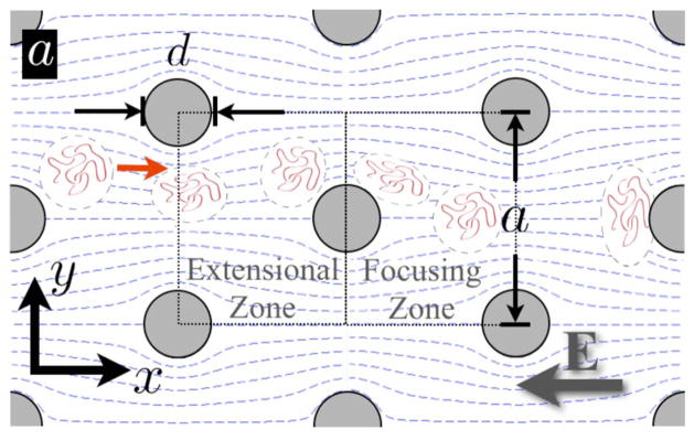
Sparse array of posts with diameter d and center-to-center spacing a. During electrophoretic transport the DNA molecules follow the dashed electric field lines. The extensional electrophoretic flow in the extensional zone leads to a deformation of the DNA that increases the probability of collision. The focusing zone after the post has electric field lines that tend to drive the DNA into a position that favors collisions with the next post. Reprinted with permission from Ref. Copyright 2009 The American Physical Society.
Size exclusion chromatography separation of DNA in a post array. (a) Principle of the size exclusion process. (b) SEM image of the post array. (c) Electropherogram for a separation voltage of 40 V and a separation length of 4 mm. Reprinted with permission from Ref. Copyright 2003 American Institute of Physics.
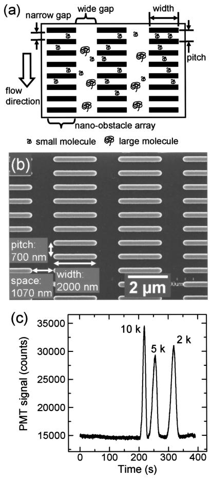
Slit-well motifs for exploiting (a) the entropic trapping regime using long DNA and (b) the Ogston sieving regime using short DNA. (c) The devices are patterned by two etching steps. As we see from the side view of the device (90° rotation of the other schematics), the optical lithography patterning of the devices leads to similar periodicities and channel sizes in both types of devices. The direction of the DNA motion is the same in panels (a) and (b).
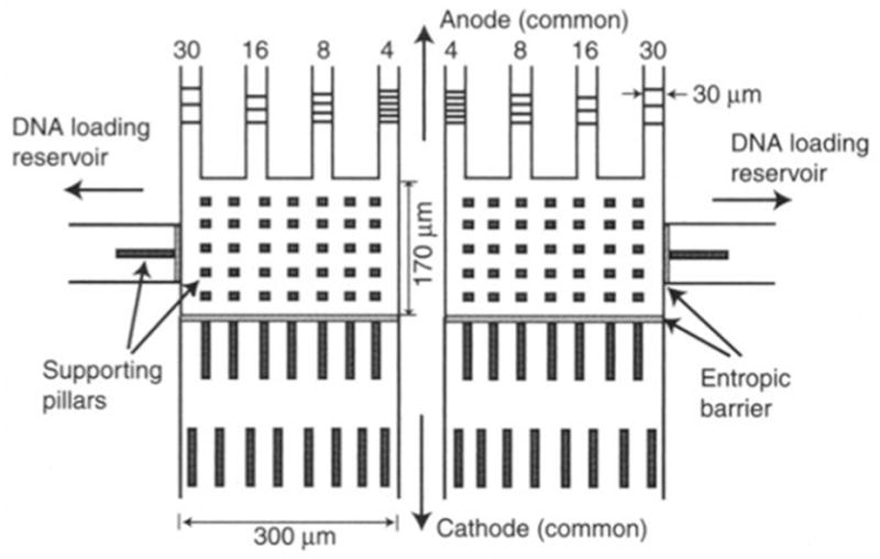
Schematic of the multilane separation device for entropic trapping. All eight channels are connected to a common anode and cathode. Each set of four arrays is connected to their own DNA loading zone. This allows for two different mixtures to be separated simultaneously, similar to a submarine gel electrophoresis setup. Reprinted with permission from Ref. Copyright 2000 American Association for the Advancement of Science.
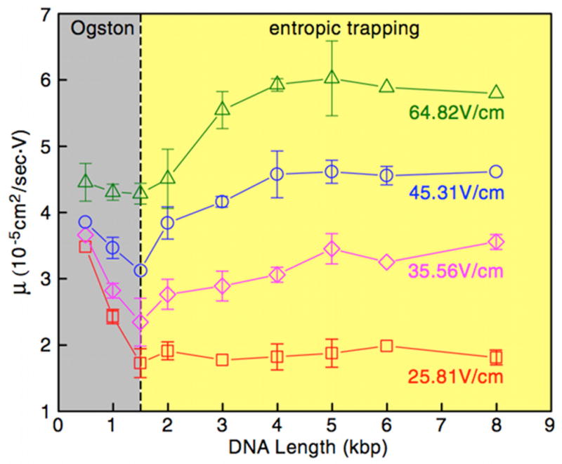
Mobility as a function of DNA length at several electric fields in the DNA nanofilter. This figure illustrates the transition from the Ogston regime, where the mobility decreases with length, to the entropic trapping regime, where the mobility increases with molecular weight. Reprinted with permission from Ref. Copyright 2006 American Physical Society.
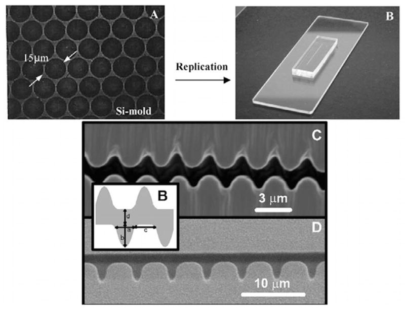
Images of the PDMS devices for entropic trapping. The top two images are a post array device, where (A) is an SEM of the silicon mold and (B) is a photograph of the final device. Reprinted with permission from Ref. Copyright 2003 Elsevier Science B.V. The bottom panel are SEM images of structured channels, with the inset defining the dimensions of the structures. Reprinted with permission from Ref. Copyright 2003 Elsevier Science B.V.
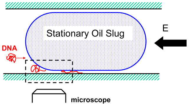
Schematic of the oil slug in the microchannel. The region between the wall of the channel and the oil slug creates a nanoslit. The interface between the channel and the nanoslit causes the DNA molecule to stretch. Reprinted with permission from Ref. Copyright 2008 American Institute of Physics.
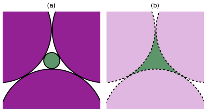
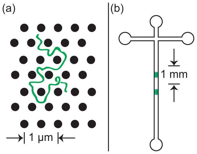
(a) The space available to a DNA molecule in a close-packed plane (purple) when one attempts to fit a solid sphere (green) into the interstitial space. (b) The space actually available to a DNA molecule in a random conformation. The actual three-dimensional network available to the molecule is much more complex than illustrated in this two dimensional projection.
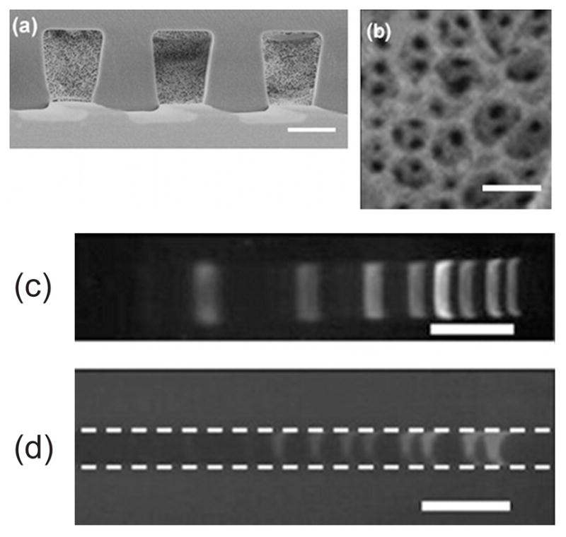
(a) A side-on SEM of the inverse opal, fabricated from SU-8. This image shows three parallel channels. These are not the channels used for the separations. (b) Close-up of the porous structure, which is analogous to an agarose gel network. The scale bar in (a) and (b) is 400 nm. (c) Bands from electrophoresis of a 1 kbp ladder in an agarose gel. (d) Bands from electrophoresis of a 1kbp ladder in an inverse opal. The dashed lines represent the walls of the microchannel. The scale bar in (c) and (d) is 1 cm. Figure reproduced with permission from Ref. Copyright 2007 Elsevier B.V.
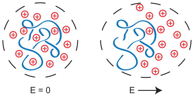
Schematic illustration of the polarization of a DNA/counterion system. In the absence of the electric field, the system in the dashed lines is electroneutral and unpolarized. For clarity, only the DNA (negatively charged) and the counterions (positively charged) are shown. Immediately after the application of an electric field, the counterions move in the direction of the electric field and the DNA moves in the opposite direction. The system in the dashed lines is still electroneutral but it is now polarized. The polarization only exists on a time scale that is short compared to the relaxation time of the counterions. After longer times, the flux of counterions from left-to-right replenishes the lost counterions on the left hand side while maintaining electroneutrality. Thus, in a steady uniform electric field, the DNA/counterion cloud is unpolarized and the motion is due to electrophoresis.
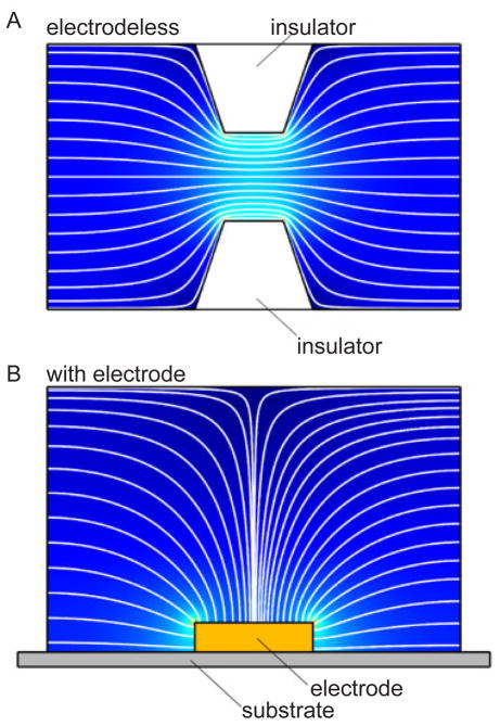
Schematic illustration of (A) the electric field produced by a constriction in an insulator and (B) the electric field proximate to an electrode. Reprinted with permission from Ref. Copyright 2011 Wiley-VCH.
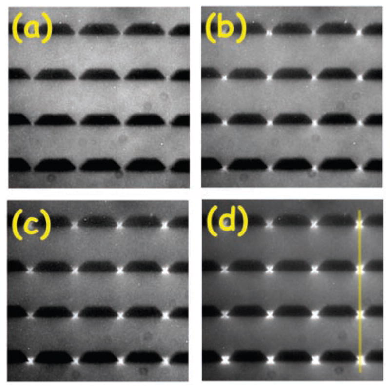
Dielectrophoretic trapping of 386 bp DNA using a voltage of 1 kV (5 V peak-to-peak across each unit cell) with applied frequencies of (a) 200 Hz, (b) 400 Hz, (c) 800 Hz, and (d) 1000 Hz. The frame size is 80 × 80 μ m. The vertical line in (d) refers to a later figure in Ref. Reprinted with permission from Ref. Copyright 2002 Biophysical Society.
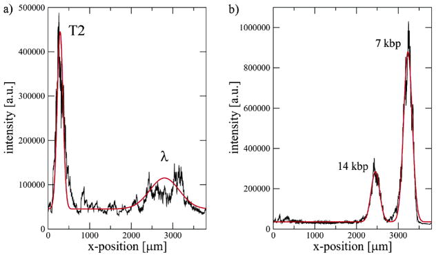
Electropherograms for the dielectrophoretic separation of DNA using a gradual increase in the strength of the ac electric field. The black lines are the raw data and the red lines are fits. In both cases, a steady field with a 12 V drop across the channel provides the dc electrophoretic motion and the ac field has a frequency of 60 Hz. (a) Separation of λ DNA (48.5 kbp) and T2 DNA (164 kbp). The ac field increases from 150 V in 0.6 V increments every 3 seconds until reaching 189 V. (b) Separation of a 7 kbp closed circular plasmid and its 14 kbp dimer. The ac field increases from 198 V in 6 V increments every 30 seconds until reaching 240 V. Reprinted with permission from Ref. Copyright 2007 American Chemical Society.
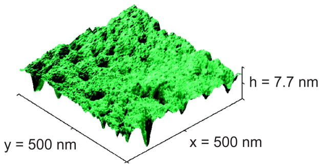
Atomic force microscope (AFM) image of the surface of the channels used in 20 nm nanoslit DNA electrophoresis experiments measured using a 2 nm radius tip. The rms roughness is between 0.8 to 1.1 nm but the maximum hole depth is 8 nm. Reprinted with permission from Ref. Copyright 2008 American Chemical Society.
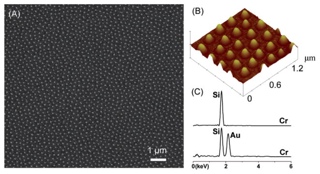
(A) Scanning electron microscopy (SEM) image of gold nanodots on a Si surface. (B) Atomic force microscope image of the same system. (C) Energy dispersion analysis of the bare Si and the Si/Au regions, respectively. Reprinted with permission from Ref. Copyright 2006 American Chemical Society.
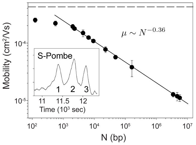
Mobility as a function of DNA size for surface electrophoresis on silicon with a hexagonal pattern of nickel spots. The dashed line at the top is the free solution mobility. The inset shows the separation of three chromosomes from S. Pombe (1 =3.5 Mbp 2 = 4.7 Mbp 3 = 57 Mbp). Adapted with permission from Ref. Copyright 2004 American Chemical Society.
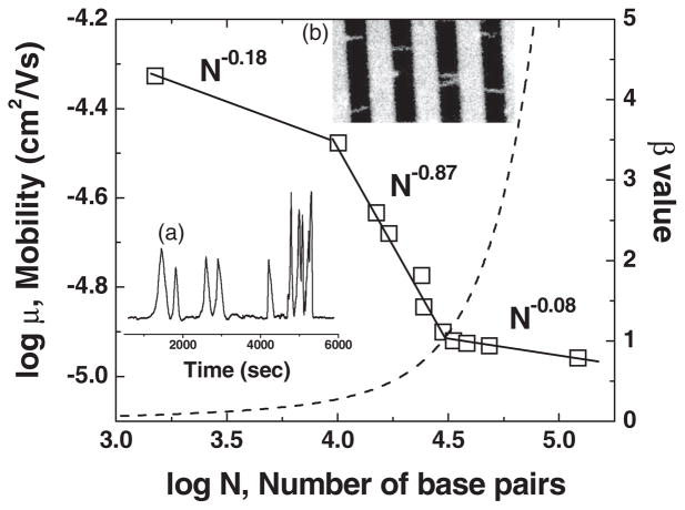
Mobility versus molecular weight for surface electrophoresis on an Au striped surface with a spacing of 3 μ m. The dashed curve is a prediction for a parameter β that is related to the stretching of the DNA from a simple model described in Ref. Inset (a) is an electropherogram for the λ DNA MonoCut mix. Inset (b) is an image of DNA trapped on the surface pattern with an 8 μ m spacing. Reprinted with permission from Ref. Copyright 2007 American Physical Society.
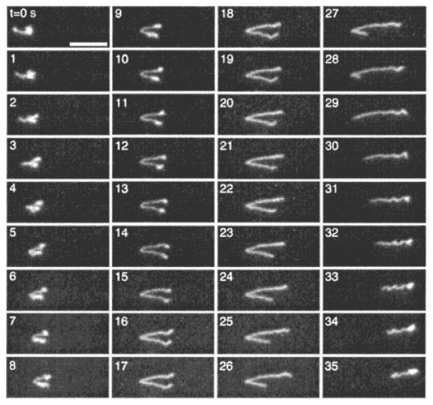
Sequence of images of λ DNA hooking on lipids during electrophoresis in a lipid bilayer at E = 3.3 V/cm. The scale bar is 10 μ m and the times for each image are listed in seconds. Reprinted with permission from Ref. Copyright 2001 American Chemical Society.
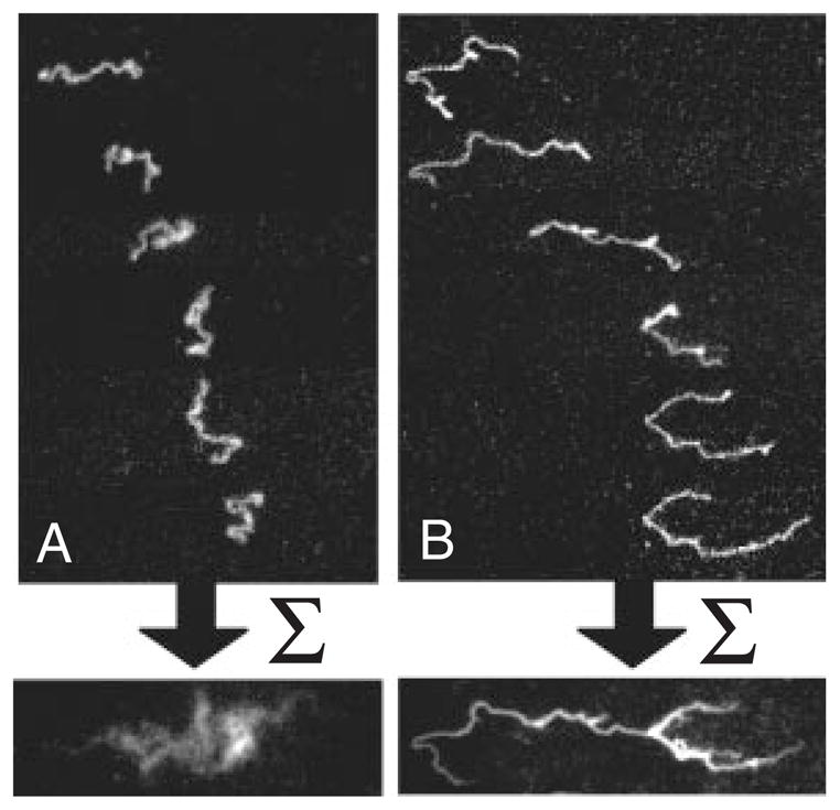
Videomicroscopy images of DNA electrophoresis on a cationic lipid bilayer. The snapshots in (A) correspond to an electric field of 0.2 V/cm and the snapshots in (B) correspond to an electric field of 10 V/cm. The image at the bottom is the time average of each series. Reprinted with permission from Ref. Copyright 2009 Wiley-VCH.
A separation of two different sized DNA molecules performed in a continuous separation device. The band with the larger defection angle is the smaller DNA. (A) No tilt, high speed. (B) No tilt, low speed. (C) Tilted, low speed. Species (a) is 164 kbp and species (b) is 48.5 kbp. Adapted with permission from Ref. Copyright 2003 American Chemical Society.
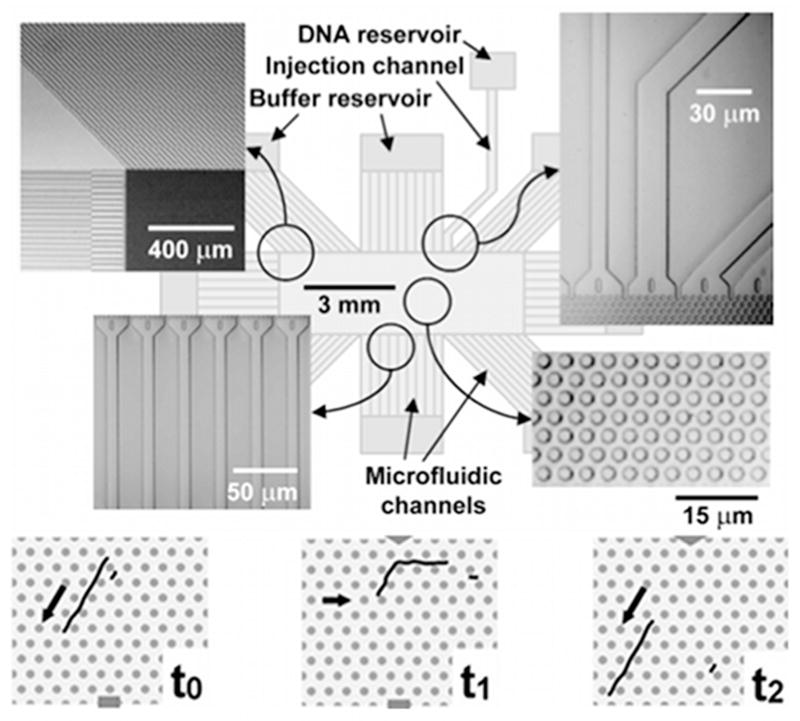
Top: Schematic of the DNA prism. The SEM images in the insets highlight different regions of the device. Bottom: Illustration of the separation mechanism. At t0 both the long and short fragment travel in the strong field direction. At t1 the field is switched to the weak field in a new direction. The long DNA molecule cannot get all the way around the corner, but the smaller molecule can. At t2 the field is switched back to the strong field and the long DNA travel down the same channel while the shorter DNA is now in a new channel. Reprinted with permission from Ref. Copyright 2002 Nature Publishing Group.
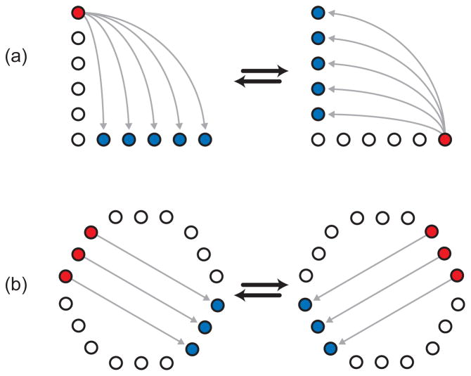
Schematic illustration of the anisotropic nanofilter array (ANA). (a) For the Ogston sieving regime, where the radius of gyration is smaller than the gap, the smaller molecule has a higher rate of crossing the gap. (b) For the entropic trapping regime, where the radius of gyration is larger than the gap, the larger molecule has a higher rate of crossing the gap. This image is for the planar ANA device, but the same idea holds for the vertical device. Adapted with permission from Ref. Copyright 2007 Nature Publishing Group.
A image of the Brownian ratchet. For the molecule to travel from the gap it is in to the adjacent gap to the right, it needs to move from the gap to the start of the next tilted obstacle, about 1.5 μm. To move to the left gap the molecule needs to travel the entire distance of the obstacle, about 5 μm, or be shunted back to the gap it started at by the obstacle. It also has less time to diffuse left before colliding with the obstacle. Practically, no molecules travel to the left. Reprinted with permission from Ref. Copyright 1999 National Academy of Sciences of the U.S.A.
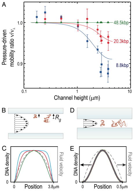
(a) Relative velocity as a function of nanoslit height, h. (b) Schematic illustration of hydrodynamic chromatography for h ≫ Rg. (c) Prediction from a random flight model for the density of DNA segments as a function of molecular weight. The color coding is the same as in (a). (d) Schematic illustration of the DNA configurations for h = 3.81 μm. (e) Prediction from a random flight model for the density of DNA segments as a function of molecular weight for h = 500 nm. The color coding is the same as in (a). In (c) and (e), the fluid profile is indicated in gray. Modified with permission from Ref. Copyright 2006 The National Academy of Sciences of the U.S.A.
Hydrodynamic chromatography of DNA in a 2.5 μm inner diameter, 445 cm long capillary under a pressure of 360 psi in a 10 mM Tris, 1 mM EDTA buffer. Reprinted with permission from Ref. Copyright 2010 American Chemical Society.
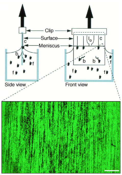
Schematic of molecular combing process. The silanized surface of the glass selectively attaches the 5′ end of the DNA, and the moving air-water contact line stretches and fixes the DNA molecule to the surface. DNA is represented in the figure as free-solution (f), bound (b), combed (c) and looped (lo) — when both ends bind to the surface. The scale bar is 25 μm. Adapted with permission from Ref. Copyright 1997 American Association for the Advancement of Science.
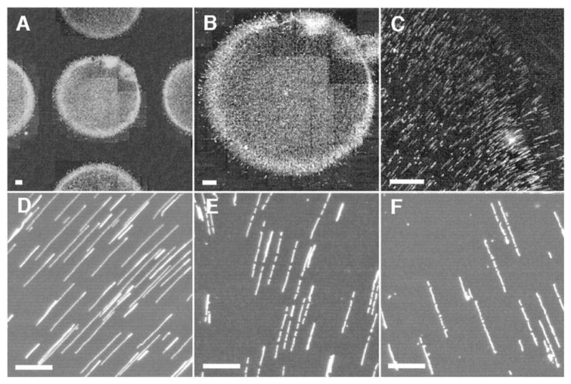
Fluid fixing of DNA on APTES-treated glass surfaces. The drying process produces a high degree of alignment within the spot. Spotting these droplets with an automated process facilitates automated image analysis of fragment sizes. Scale bars represent 20 μm in (A–C) and 5 μm in (D–F). Adapted with permission from Ref. Copyright 1998 National Academy of Sciences of the U.S.A.
Surface stretching via microfluidic channels yields highly aligned DNA on the surface. (a) PDMS microchannel. (b–e) Montages of stretched DNA using adenovirus DNA (b), λ DNA 9c), RS281 DNA (d) and T2 DNA (e). (f–i) Magnification of small segments of images (b)–(e). Reprinted with permission from Ref. Copyright 2004 American Chemical Society.
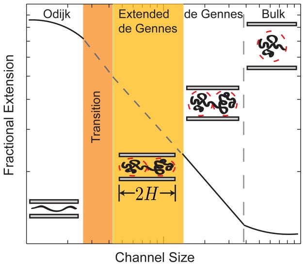
Qualitative sketch of the regimes of extension for a DNA chain as a function of the channel size D. The schematics show the qualitative models for the configurations of a confined chain. Adapted with permission from Ref. Copyright 2011 American Chemical Society.
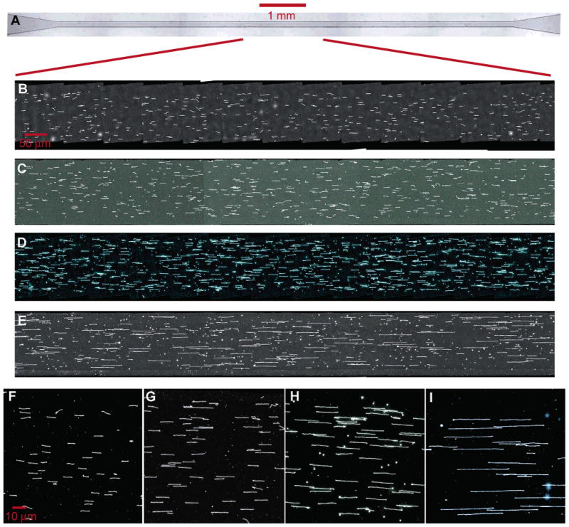
Device design for loading DNA into channels in the Odijk regime. (a) SEM micrograph of 85 nm nanochannels made by nanoimprint lithography that are subsequently thinned to channels on the order of 10 nm. The scale bar is 500 nm. Also included is the diffraction gradient lithography schematic (right), showing the gradual slope change approaching the nanochannels. (b) Schematic of microchannel-nanochannel interface (top), and fluorescence micrograph of the loading process. Adapted with permission from Ref., Copyright 2002 American Institute of Physics.
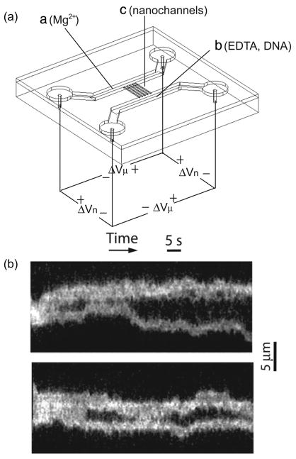
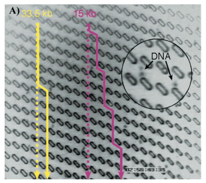
(a) Schematic of nanochannel device for ordered restriction mapping. Note the separate locations for loading the DNA and loading the restriction enzyme co-factor Mg2+. (b) Time-resolved restriction maps of single PacI cut of a 61 kbp DNA PAC insert. Adapted with permission from Ref. Copyright 2005 National Academy of Sciences of the U.S.A.
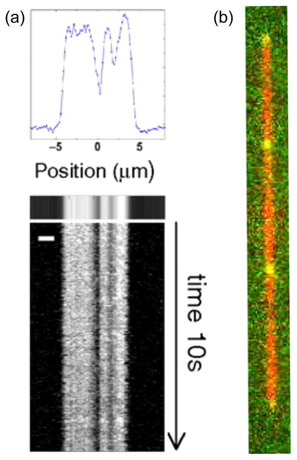
(a) Local melting maps (scale bar is 2 μm) for λ DNA at 28°C. Adapted with permission from Ref. Copyright 2010 National Academy of Sciences of the U.S.A. (b) DNA barcoding showing two colors, one for the backbone dye and a second for the internal probes. Adapted with permission from Ref. Copyright 2011 Su et al. and subject to the Creative Commons Attribution License.
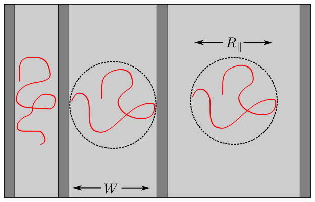
Polymer confinement in a nanochannel (left), high-aspect ratio nanochannel at the critical point where the slit width, W, equals the in plane radius of gyration (center), and a slit with true quasi-2D confinement (right). In this image, the chain is strongly confined in the direction perpendicular to the page.
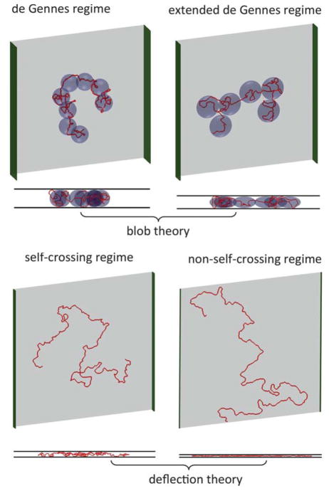
Four regimes of confinement in a nanoslit that appear to explain the existence of a broad transition in slit extension from the classical de Gennes regime to the Odijk regime. Adapted with permission from Ref. Copyright 2012 Royal Society of Chemistry.
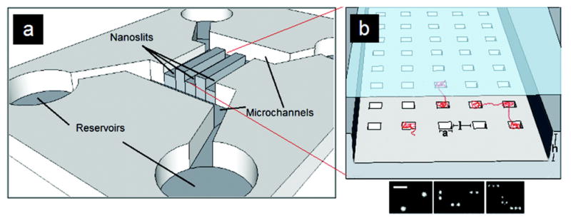
Schematic of the (a) chip design and microchannels and (b) nanoslit and nanopit array for a nanopit entropic trap. Adapted with permission from Ref. Copyright 2012 American Chemical Society.
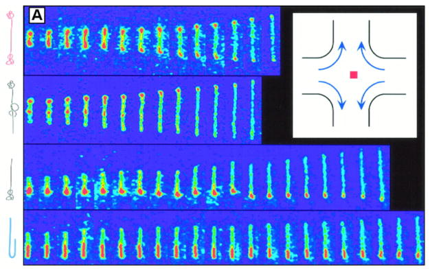
Fluorescence microscopy images of λ DNA stretching in an extensional flow with an extensional rate ε̇ = 0.86 s−1. The images are spaced at 0.13 s intervals. The dynamics of the stretching depend strongly on the initial conformation of the chain, which is sketched at the left hand side of the image. The inset is a schematic image of the extensional flow in a cross-slot channel. Reprinted with permission from Ref. Copyright 1997 American Association for the Advancement of Science.
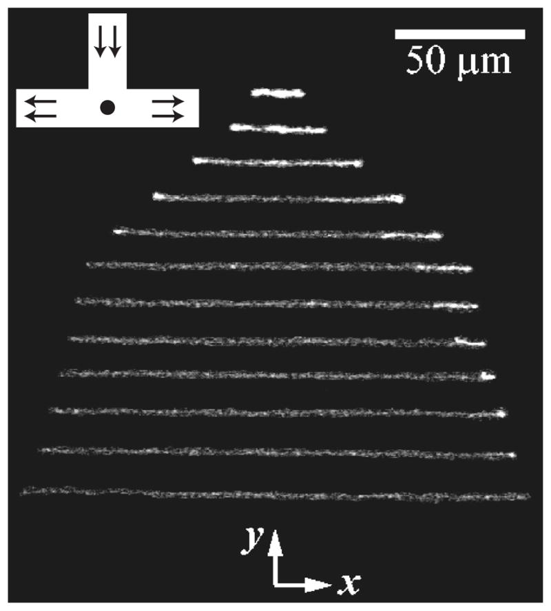
Images of the stretching of a 10-λ concatemer (485 kbp) in an extensional electric field created at a T-junction. The images are separated by 0.33 seconds. The inset is a schematic of the T-junction, with the stagnation point indicated by the circle. Modified with permission from Ref. Copyright 2007 American Institute of Physics.
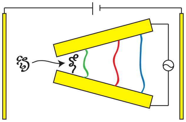
Principle behind a dielectrophoresis sizing device. Two electrodes are placed at an angle to one another to create local maxima in the electric field gradient near each of the electrodes. An ac field is applied between these two electrodes, so that any DNA molecules between the electrodes tends to be stretched between them. The DNA enter the gap between these electrodes by dc electrophoresis or a fluid flow.
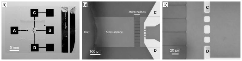
Device for single molecule insertion and stretching of DNA molecules by dielectrophoresis. (a) Photograph of the overall device. The dc electric field is applied between pads A and B, and the ac electric field is applied between pads C and D. (b) View of the active region of the device. The access channel is 300 μ m wide and the microchannels are 1 μ m wide. The channels are 4 μ m deep. (c) DNA stretching region. The voltage is applied between electrode C and D, and the DNA are stretched between the isolated metal spots on the surface. Reprinted with permission from Ref. Copyright 2007 Wiley-VCH.
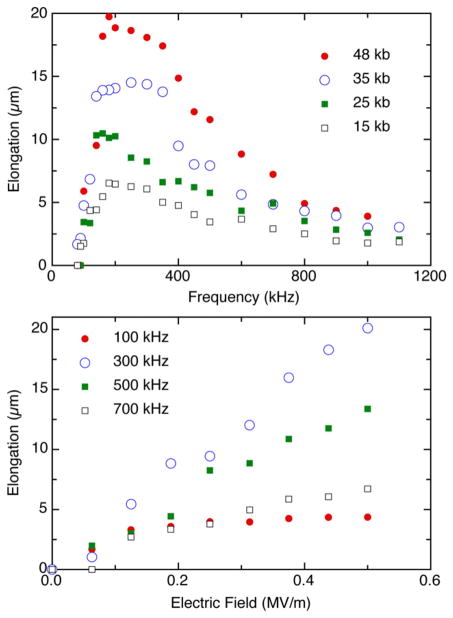
Elongation of DNA by dielectrophoresis in a 40 μ m wide gap between two electrodes. Top: Extension as a function of frequency for different molecular weights. Bottom: Extension of λ DNA as a function of electric field strength for different frequencies. Reprinted with permission from Ref. Copyright 2006 IOP Publishing Ltd.
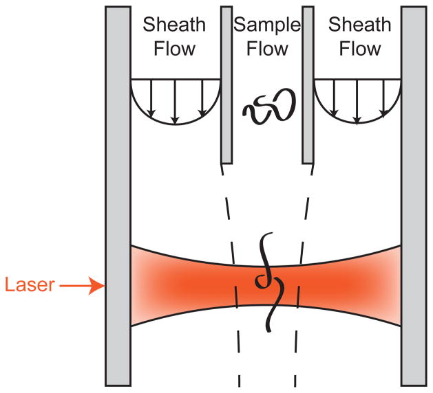
Schematic illustration of the principle of flow cytometry for sizing DNA. The sheath flow focuses the sample stream as it flows towards the laser excitation. Dashed lines demarcating the boundary between fluid elements in the sheath flow and the sample flow are included to illustrate the flow focusing concept. The laser induced fluorescence detection is normally performed at a 90° angle with respect to the excitation.
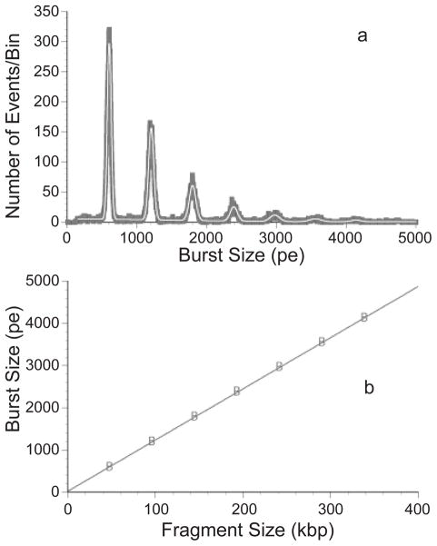
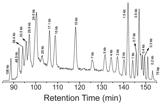
Linear response of fluorescence burst analysis in flow cytometry with the size of the DNA. (a) Histogram of the burst sizes (in bins of 10 photoelectrons, pe) for concatemers of λ DNA (48.5 kbp) up to 7-λ (339.5 kbp). The dark line is the raw data; the white line is the sum of seven Gaussian functions fit to the data. The frequency of large concatemers is very low. (b) Linearity of the response in the burst size with respect to the size of the DNA fragments. The correlation coefficient is 0.99998. Reproduced from Ref. with permission. Copyright 1999 Wiley-Liss, Inc.
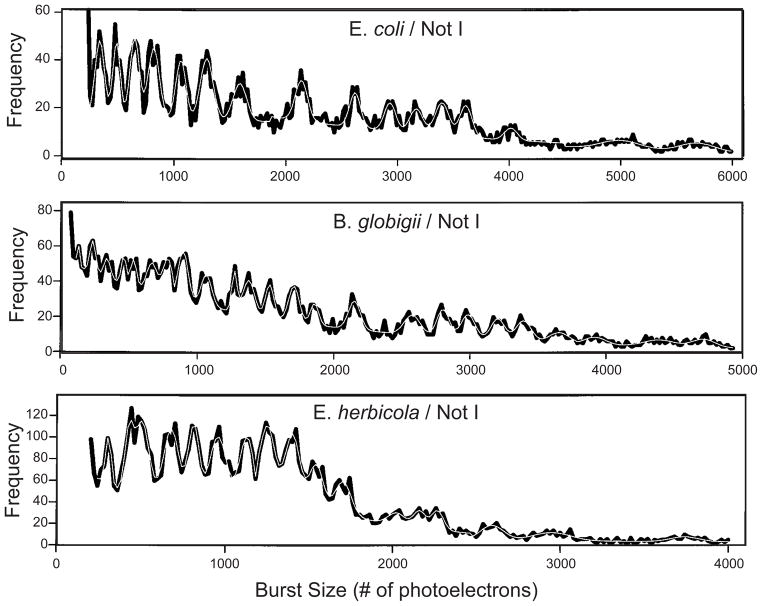
Flow cytometry burst histograms for the NotI fingerprints of three different organisms. The black lines are the raw data and the white lines are the sum of Gaussian fits to the data. Adapted with permission from Ref. Copyright 1999 Wiley-Liss, Inc.
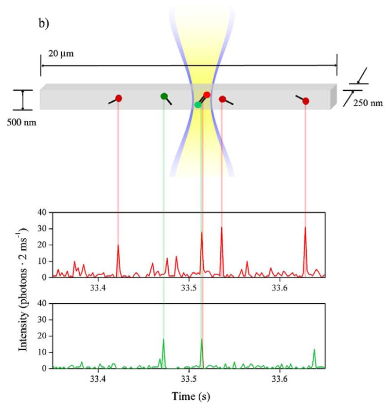
Illustration of the principle of two color analysis of DNA in cytometry device. These particular experiments were performed in a submicron channel using electrophoretic cytometry, which is discussed in more detail in Section 8.2. Reprinted with permission from Ref. Copyright 2007 American Institute of Physics.
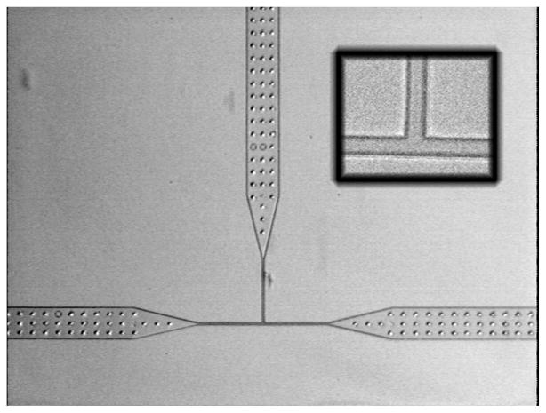
Microfluidic flow cytometer for DNA fabricated in PDMS. The inset is a magnified image of the intersection of the channels. The large channels are 100 μm wide and narrow to 5 μm at the junction. The channels are 3 μm deep. The pillars in the wide channels support the ceiling of the channel. Reprinted with permission from Ref. Copyright 2009 National Academy of Sciences of the U.S.A.
Artistic rendition of direct linear analysis device from US Genomics. Reprinted with permission from Ref. Copyright 2004 Creative Commons License.
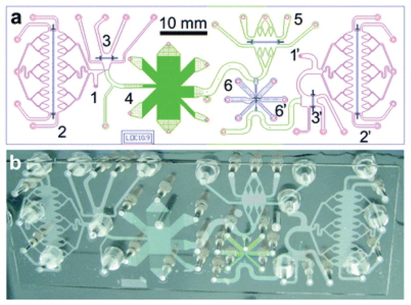
Highly integrated device that combines separations, DNA stretching, and fluorescence burst analysis. (a) Schematic illustration of the device. (b) Actual device. The various numbered components of the device are described in the original reference. Note that component 4 is a DNA prism. Reprinted with permission from Ref. Copyright 2011 Royal Society of Chemistry.
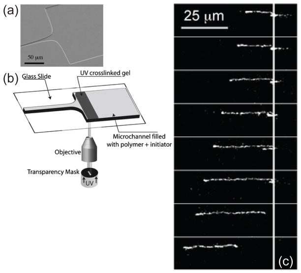
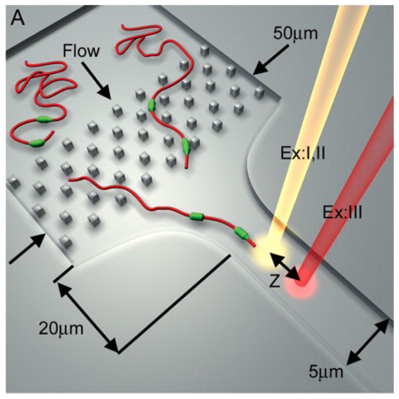
(a) Hyperbolic contraction similar to the system in Figure 75. (b) Illustration of the experimental protocol for creating a gel near the entrance to the hyperbolic contraction. (c) Images of the DNA extension as it crosses from the gel into the fluid before the hyperbolic contraction. The solid line indicates the location of the gel/fluid interface. Reprinted with permission from Ref. Copyright 2006 Royal Society of Chemistry.
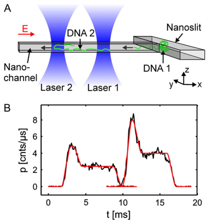
(a) Schematic illustration of the two laser-spot device for DNA electrophoretic cytometry in a nanochannel. (b) Trace of the intensity output through the laser spots for a folded DNA molecule. Reprinted with permission from Ref. Copyright 2008 Biophysical Society.
References
Publication types
MeSH terms
Substances
Grants and funding
LinkOut - more resources
Full Text Sources
Other Literature Sources
