. 2013 Jan;37(1):63-79.
doi: 10.1111/ejn.12021. Epub 2012 Nov 21.

Nonassociative plasticity alters competitive interactions among mixture components in early olfactory processing

Affiliations

Nonassociative plasticity alters competitive interactions among mixture components in early olfactory processing

Fernando F Locatelli et al. Eur J Neurosci. 2013 Jan.

Abstract

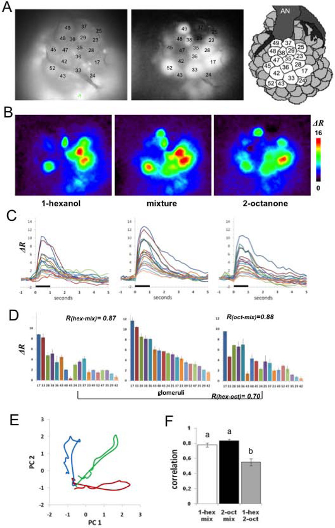
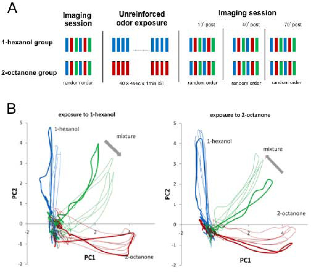
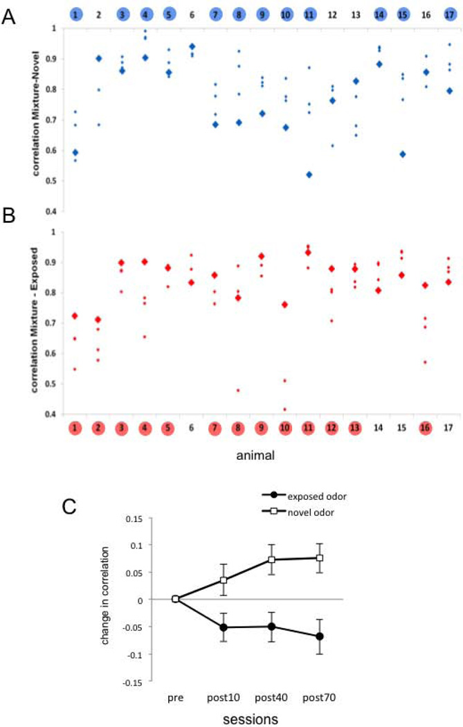
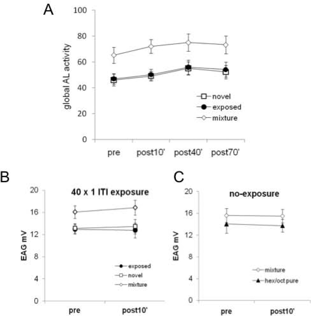
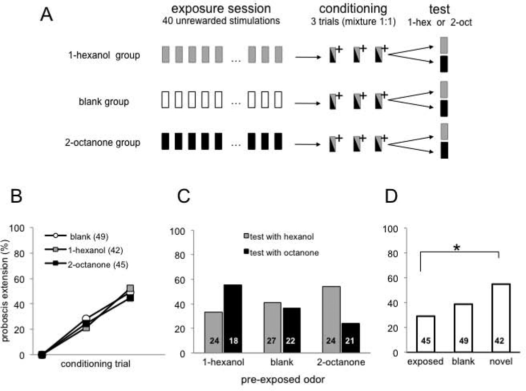
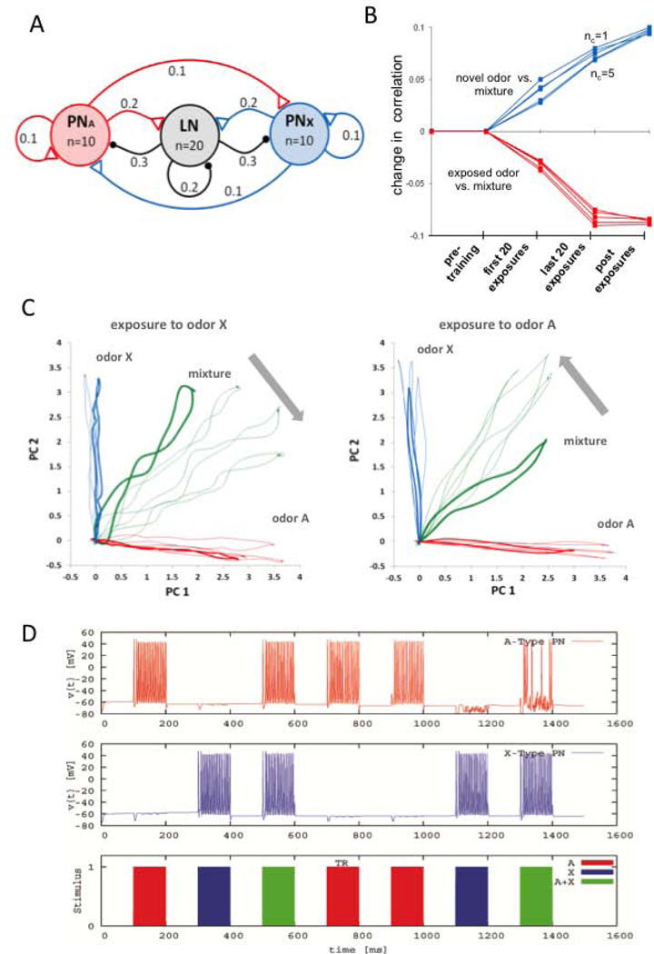
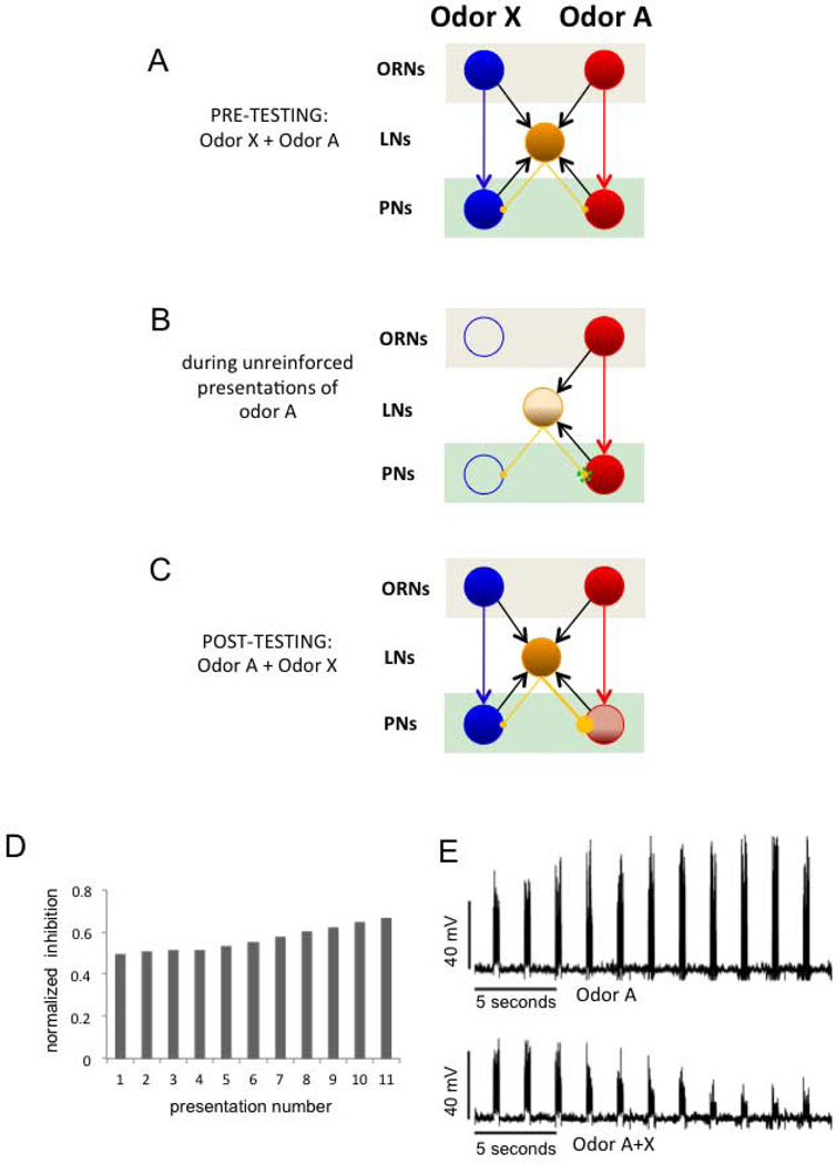
Experience-related plasticity is an essential component of networks involved in early olfactory processing. However, the mechanisms and functions of plasticity in these neural networks are not well understood. We studied nonassociative plasticity by evaluating responses to two pure odors (A and X) and their binary mixture using calcium imaging of odor-elicited activity in output neurons of the honey bee antennal lobe. Unreinforced exposure to A or X produced no change in the neural response elicited by the pure odors. However, exposure to one odor (e.g. A) caused the response to the mixture to become more similar to that of the other component (X). We also show in behavioral analyses that unreinforced exposure to A caused the mixture to become perceptually more similar to X. These results suggest that nonassociative plasticity modifies neural networks in such a way that it affects local competitive interactions among mixture components. We used a computational model to evaluate the most likely targets for modification. Hebbian modification of synapses from inhibitory local interneurons to projection neurons most reliably produced the observed shift in response to the mixture. These results are consistent with a model in which the antennal lobe acts to filter olfactory information according to its relevance for performing a particular task.


Conflict of interest statement

None of the authors have a conflict of interest for this work.

Figures

Figure 1
Figure 1
Calcium imaging of projection neurons in the honey bee antennal lobe. A, View of the antennal lobe after staining the PNs. The picture shows the dorsal surface including 18 identified glomeruli (Galizia et al., 1999) used for the imaging analyses. Left: basal fluorescence images obtained with 380nM excitation light and LP510 emission filter, allow identification of glomeruli according to size, shape and position by comparison with the published honey bee AL atlas (Galizia et al., 1999; Flanagan and Mercer 1989). Basal fluorescence images are also used for verification of homogeneous staining in all glomeruli used for analysis. Middle panel: Correlation images (see methods) clearly define boundaries between glomeruli and thus were used as an additional tool to verify glomeruli identification. Darker glomeruli do not indicate lack of staining (controlled for from the images such as the one in the left panel); these glomeruli were not activated by the odors and consequently produce a low correlation values between neighboring pixels). Right panel: Schema of the dorsal surface on the honey bee AL showing 18 glomeruli used in our analyses (AN: antennal nerve). B, Color-coded (see scale) changes in calcium levels averaged between 400 and 800 ms after odor onset. The figures show distinct but slightly overlapping spatial activity patterns for each of the three odors. C, Glomerular activity over time to show spatio-temporal activity patterns. The same line color across figures represents the change in ratio over 6 s (1 s before stimulation through 5 s after) in a single identified glomerulus for each of the three odors. D, Calcium responses for each of the 18 glomeruli averaged over 1s of stimulation ordered from the highest response to the lowest for the mixture (middle figure). The same ordering was maintained for 1-hexanol (left) and 2-octanone (right) to emphasize changes in activity in each glomerulus for each of the odors compared to the mixture. Error bars represent Standard Deviation of two measurements. R-values inserted in the Fig. 1D refer to the Pearson correlation coefficients used to compare pairs of odor patterns within animal and within session. E, Principal Components Analysis (see Methods) used to show the evolution of the activity patterns over 200 ms time steps during odor stimulation in one animal (Galan et al., 2006; Fernandez et al., 2009) for 1-hexanol (blue), the mixture (green) and 2-octanone (red). With the onset of odor stimulation the transients for the pure odors project along each PC axis and reach maximal separation between 400 and 600 ms (Fernandez et al., 2009). After odor termination the transients loop back and return to origin. F, Mean +/− SE of the correlation coefficients indicated in D, for 17 animals prior to any treatment. The correlations between the pure components and the mixture are significantly higher than the correlation between the pure odorants; different letters on tops of the bars indicate significant differences at p<0.01.
Figure 2
Figure 2
Effect of odor exposure on odor-induced spatiotemporal activity in the AL. A, Experimental protocol: Each imaging session includes two stimulations each with 1-hexanol, 2-octanone and the mixture (1:1) distributed in random order and separated by 1min ISI. The exposure consisted of 40 4-sec presentations of either 1-hexanol or 2-octanone separated by 1 min inter-stimulus interval (ISI). The exposure session started 5 min after the end of the first imaging session. Odor representations were measured again in the second, third and fourth imaging session performed 10, 40 and 70 minutes after the end of the exposure, respectively. B, Odor elicited responses from 18 glomeruli are represented using Principal Component Analysis. The animals exposed to 1-hexanol (n=8) and to 2-octanone (n=9) were separately averaged to obtain two average-bees with 18 glomeruli each (Methods; Fernandez et al 2009). The 18 dimensions used to describe odor transients were reduced to its first two principal components (95% and 97 % of the total variance respectively). Bold lines indicate the first imaging session, which was done before the exposure session. Thin lines belong to the 2nd, 3rd and 4th imaging sessions performed after exposure. We use PCA for visualization only. Statistical analyses as well as conclusions are based on the absolute correlation values presented in figure 3.
Figure 3
Figure 3
Correlation coefficients between the mixture and the pure odors before and after exposure. A. Absolute Pearson correlation coefficients between the activity patterns elicited by the novel odor (odor not used during exposure) and the mixture for each individual bee (n=17). Bold blue diamonds correspond to the correlation value before exposure. Small diamonds correspond to the correlation values after exposure. Numbers highlighted in blue indicate bees in which the average of the correlation from the three post-exposure sessions is higher than the correlation in the initial session. B. Absolute Pearson correlation coefficients between the exposed odor and the mixture for each individual bee. Bold red diamonds correspond to the measurement performed before exposure and small diamonds to the measurements performed after exposure. Numbers highlighted in red indicate bees in which the average of the correlation values obtained in the three post-exposure sessions is lower than the correlation in the initial session. Statistical analysis was strictly based on raw correlation values as they are shown in figures A and B. Two factors repeated measures ANOVA; factor 1 “novel or exposed” odor, NS; factor 2 (repeated measurement) “sessions”, NS; Interaction p =0.001. C. The data from figures A and B plotted as the net change of the correlation along the experiment. The figure shows the average and SEM of the difference between each post-exposure session and the session before exposure (n=17). The change in correlation was calculated within each bee by subtracting the correlation value obtained in the first test session from the values obtained in the post-exposure sessions.
Figure 4
Figure 4
Evaluation of sensory adaptation as a possible basis for the effect in the antennal lobe. A. Global antennal lobe activity elicited by the exposed odor, the novel odor and the mixture along all sessions. The figure shows the sum of the calcium responses in the 18 measured glomeruli. No differences were found for 1-hexanol or 2-octanone exposed bees (data not shown). Data were therefore pooled for the exposed odor, novel odor or mixture and analyzed along sessions. Statistical significance p<0.01 for both pure odors against the mixture and p<0.01first session against the third, and between fourth sessions for all odors; interaction not significant. The differences reported along sessions were not specific for the exposed odor. B. EAG was performed for the mixture and the pure odors 10’ before and 10’ after the exposure protocol coincident in time with the first and second session of the imaging experiments. Responses pre- vs post- were not significantly different (n=10 bees). C, A group of animals underwent two EAG sessions separated by 60 min, with no exposure protocol in-between, but coincident in time with the first and the second session of the imaging experiment. No change between both sessions was observed (n=5 bees).
Figure 5
Figure 5
Effect of repeated odor exposure on perception of an odor mixture. A, Schema showing the experimental procedure. Exposure session: 40 unrewarded stimulations with 1-hexanol, 2-octanone or air (blank group); Conditioning session: olfactory conditioning of the proboscis extension reflex (Bitterman et al., 1983) using a 1:1 mixture (1-hexanol: 2-octanone); (+) indicates reinforcement with 0.4 µl of 2M sucrose paired with the mixture. Test session: conditioned response was tested with 1-hexanol or 2-octanone (animals were tested only once). Proboscis extension response during exposure protocol was not recorded, since these two odors do normally not elicit any response before conditioning. B, Performance during conditioning showing percentage of animals extending the proboscis to the mixture during the three training trials. Results indicate % of response during the odor period and before reward. All groups were trained identically; they differed only in regard to treatment during the exposure session before training. No difference was found for the three groups and significant effect between trials for all groups. C, Each of the three groups was split into 2 groups for testing with the pure components (1-hexanol or 2-octanone). Two-way ANOVA revealed a significant interaction between exposed odor (1-hexanol, 2-ocatanone or air) and test odor F(2,130)= 3.09 p<0.05. Numbers in the bars indicate number of animals in each test condition in each exposure group. D, Same data from C reorganized by exposed odor (1-hexanol and 2-octanone as test odors when animals had been exposed to 1-hexanol or 2-octanone, respectively); novel odor (1-hexanol and 2-octanone as test odors when animals had been exposed to 2-octanone or to 1-hexanol, respectively); or blank (1-hexanol and 2-octanone as test odors after exposure to air). * p<0.05 between exposed and novel odors.
Figure 6
Figure 6
Hebbian plasticity on LN-to-PN synapses predicts the imaging results. A, Model of the antennal lobe topology used in the computational analyses. The network consists of 20 inhibitory local interneurons (LNs) and 20 projection neurons (PNs). This population is illustrated as three clusters in the figure. The connectivity within and between the clusters is determined randomly, based on the fixed probabilities indicated on the links. Connectivity probabilities relate to individual neurons, i.e. each PN has a probability of 0.2 of connecting any neuron from the LN cluster, thus in our model each PN cluster makes approx. 40 excitatory synapses onto LNs. The synaptic conductance for each type of connection is drawn from a normal distribution (by allowing no negative conductance). The mean and the SD of these parameters were 0.1µS and 0.05 µS for within- or between-cluster synapses and 10µS and 5µS for the external stimulation. A particular odorant reaches 10 PNs. Different degrees of overlap in the representation for A and X was evaluated by introducing from 1 to 5 common PNs (not shown in the schema). A pure odor is presented by injecting current into the set of PNs corresponding to odor A or odor X; the mixture is applied to the network by applying current in both A and X. B, Change in correlation between the trajectories for the pure odors and the mixture before, during and after exposure training. The correlation is performed among ten samples (i.e., ten loops on the 2D PC plane) obtained for each category (i.e., odor A vs. mixture, and odor X vs. the mixture) and for increasing levels of overlap between odor A and odor X ranging from 1 to 5 common PNs. C, The projections of the calcium trajectories of the PNs were obtained from the simulation of the computational model where each unit (PN or LN) was expressed by a conductance-based Hudgkin-Huxley-type single-compartment model. The training was performed on the same network for both odor types. In line with the experimental protocol, the affected synaptic conductances were increased to 150% of their original values in 20 odor presentations during training. D, The model’s prediction of the membrane potential time traces for two arbitrary PNs, one from each response group. In this instance, the training is performed with odor A and all plasticity is encapsulated in the odor presentation labeled by TR.
Figure 7
Figure 7
Illustration of the simplest and most efficient mechanism for implementing filtering of uninformative odors in the AL. The schema indicates excitatory connections from ORNs to PNs and to LNs, excitatory connections PNs to LN and inhibitory connections from LNs to PNs. A, Initially, lateral inhibition is weak and symmetric. The LN (yellow) receives input from both ORNs clusters. Since inhibitory connections are symmetric, the mixture induces a balanced representation of A and X across PNs. B, Hebbian potentiation of inhibitory synapses during odor exposure. During training the connections from the LN to the PNs that are simultaneously active increase their synaptic strength. C, the LN receives input from both ORNs clusters and the inhibitory connection with PN-A was potentiated. When the odor mixture A+X is presented, the PNs responding to A become silent due to the increase of the overall inhibition arriving into those PNs as a result of training. As consequence, the blue (X) odor is more strongly represented in the pattern elicited by the mixture. In other words, odor A+X recruits a higher level of synaptic inhibition into the group A than group X. D, The fraction of total inhibition on the odor-A PN group versus the total inhibition in the system after consecutive odor A presentations in B. E, Average membrane potential of the odor A PN population for several presentations of that odor. The upper figure is the response when only odor A is presented. The lower figure shows the diminishing response in the same A group during successive presentations of the A+X mixture.

Similar articles

Cited by

References

    1. Abel R, Rybak J, Menzel R. Structure and response patterns of olfactory interneurons in the honeybee, Apis mellifera. J. Comp. Neurol. 2001;437:363–383. - PubMed
    1. Ashraf SI, McLoon AL, Sclarsic SM, Kunes S. Synaptic protein synthesis associated with memory is regulated by the RISC pathway in Drosophila. Cell. 2006;124:191–205. - PubMed
    1. Bazhenov M, Stopfer M, Rabinovich M, Abarbanel HD, Sejnowski TJ, Laurent G. Model of cellular and network mechanisms for odor-evoked temporal patterning in the locust antennal lobe. Neuron. 2001;30:569–581. - PMC - PubMed
    1. Bitterman ME, Menzel R, Fietz A, Schafer S. Classical conditioning of proboscis extension in honeybees (Apis mellifera) J. Comp. Psychol. 1983;97:107–119. - PubMed
    1. Chandra SB, Wright GA, Smith BH. Latent inhibition in the honey bee, Apis mellifera: Is it a unitary phenomenon? Anim. Cogn. 2010;13:805–815. - PubMed

Publication types