

Internal representations of temporal statistics and feedback calibrate motor-sensory interval timing
- PMID: 23209386
- PMCID: PMC3510049
- DOI: 10.1371/journal.pcbi.1002771
Internal representations of temporal statistics and feedback calibrate motor-sensory interval timing
Abstract
Humans have been shown to adapt to the temporal statistics of timing tasks so as to optimize the accuracy of their responses, in agreement with the predictions of Bayesian integration. This suggests that they build an internal representation of both the experimentally imposed distribution of time intervals (the prior) and of the error (the loss function). The responses of a Bayesian ideal observer depend crucially on these internal representations, which have only been previously studied for simple distributions. To study the nature of these representations we asked subjects to reproduce time intervals drawn from underlying temporal distributions of varying complexity, from uniform to highly skewed or bimodal while also varying the error mapping that determined the performance feedback. Interval reproduction times were affected by both the distribution and feedback, in good agreement with a performance-optimizing Bayesian observer and actor model. Bayesian model comparison highlighted that subjects were integrating the provided feedback and represented the experimental distribution with a smoothed approximation. A nonparametric reconstruction of the subjective priors from the data shows that they are generally in agreement with the true distributions up to third-order moments, but with systematically heavier tails. In particular, higher-order statistical features (kurtosis, multimodality) seem much harder to acquire. Our findings suggest that humans have only minor constraints on learning lower-order statistical properties of unimodal (including peaked and skewed) distributions of time intervals under the guidance of corrective feedback, and that their behavior is well explained by Bayesian decision theory.
Conflict of interest statement
The authors have declared that no competing interests exist.
Figures
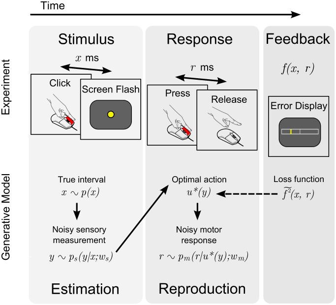
 ms later at the center of the screen, with
  drawn from a block-dependent distribution (estimation phase). The subject then pressed the mouse button for a matching duration of
  ms (reproduction phase). Performance feedback was then displayed according to an error map
  . Bottom: Generative model for the time interval reproduction task. The interval
  is drawn from the probability distribution
  (the objective distribution). The stimulus induces in the observer the noisy sensory measurement
  with conditional probability density
  (the sensory likelihood), with
  a sensory variability parameter. The action
  subsequently taken by the ideal observer is assumed to be the ‘optimal’ action
  that minimizes the subjectively expected loss (Eq. 1);
  is therefore a deterministic function of
  ,
,  . The subjectively expected loss depends on terms such as the prior
  and the loss function (squared subjective error map
  ), which do not necessarily match their objective counterparts. The chosen action is then corrupted by motor noise, producing the observed response
  with conditional probability density
  (the motor likelihood), where
  is a motor variability parameter.
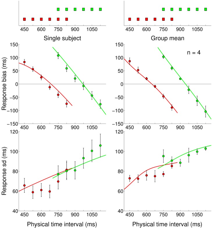
 s.e.m. across subjects). Continuous lines represent the Bayesian model ‘fit’ obtained averaging the predictions of the most supported models across subjects.
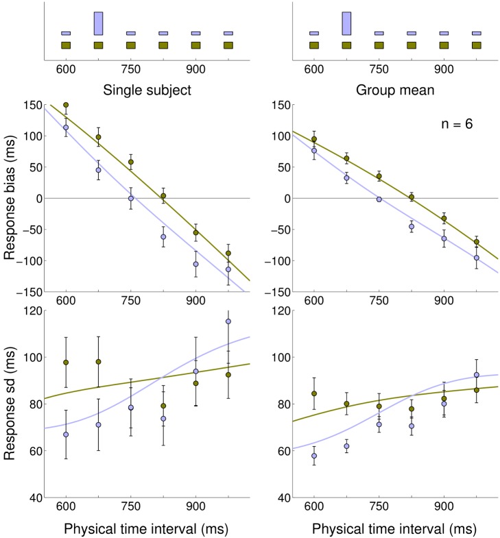
 s.e.m. across subjects). Continuous lines represent the Bayesian model ‘fit’ obtained averaging the predictions of the most supported models across subjects.
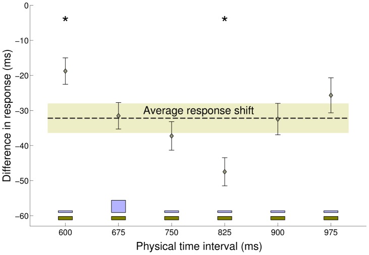
 s.e.m.). The experimental distributions (light brown: Medium Uniform; light blue: Medium Peaked) are plotted for reference at bottom of the figure. The dashed black line represents the average response shift (difference in response between blocks, averaged across all subjects and stimuli), with the shaded area denoting
  s.e.m. The average response shift is significantly different from zero (
 ms; two-sample t-test
  ), meaning that the two conditions elicited consistently different performance. Additionally, the responses were subject to a ‘local’ (i.e. interval-dependent) modulation superimposed to the average shift, that is, intervals close to the peak of the distribution (675 ms) were attracted towards it, in addition to the average shift, while intervals far away from the peak were less affected. (*) The response shift at 600 ms and 825 ms is significantly different from the average response shift;
  .
.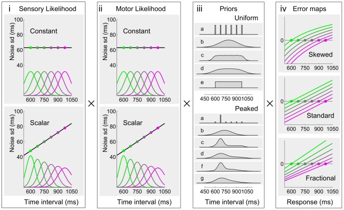
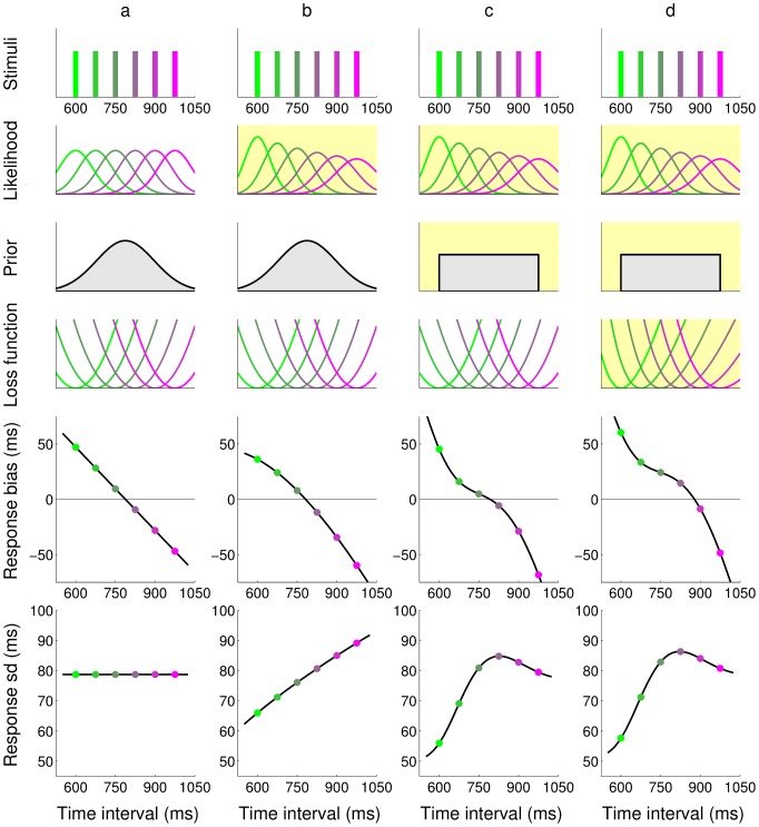
 (resp.
  ). iii) Candidate priors for the Medium Uniform (top) and Medium Peaked (bottom) blocks. The candidate priors for the Short Uniform (resp. Long Uniform) blocks are identical to those of the Medium Uniform block, shifted by 150 ms in the negative (resp. positive) direction. See Methods for a description of the priors. iv) Candidate subjective error maps. The graphs show the error as a function of the response duration, for different discrete stimuli (drawn in different colors). From top to bottom: Skewed error
  ; Standard error
  ; and Fractional error
  . The scale is irrelevant, as the model is invariant to rescaling of the error map. The squared subjective error map defines the loss function (as per Eq. 1).
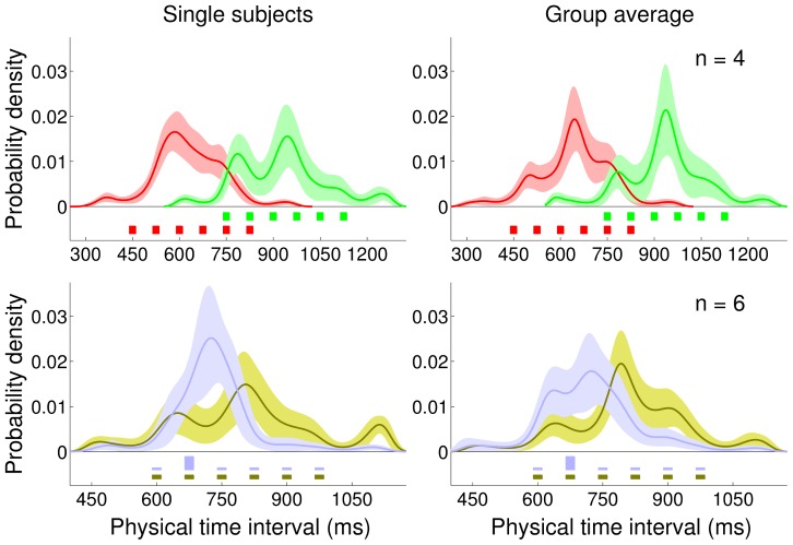
 s.d. For comparison, the discrete experimental distributions are plotted under the inferred priors.
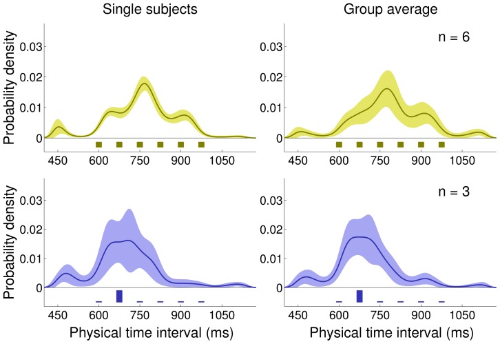
 s.d. For comparison, the discrete experimental distributions are plotted under the inferred priors.
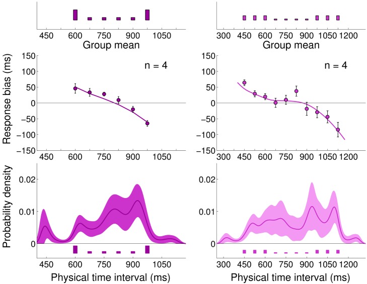
 s.e.m. across subjects) for the Medium Bimodal (left) and Wide Bimodal (right) blocks. Continuous lines represent the Bayesian model ‘fit’ obtained averaging the predictions of the most supported models across subjects. Bottom: Average inferred priors for the Medium Bimodal (left) and Wide Bimodal (right) blocks. Shaded regions are
  s.d. For comparison, the experimental distributions are plotted again under the inferred priors.
References
-
- Mauk MD, Buonomano DV (2004) The neural basis of temporal processing. Annu Rev Neurosci 27: 307–340. - PubMed
-
- Buhusi C, Meck W (2005) What makes us tick? Functional and neural mechanisms of interval timing. Nat Rev Neurosci 6: 755–765. - PubMed
-
- Miyazaki M, Nozaki D, Nakajima Y (2005) Testing bayesian models of human coincidence timing. Journal of neurophysiology 94: 395–399. - PubMed
-
- Miyazaki M, Yamamoto S, Uchida S, Kitazawa S (2006) Bayesian calibration of simultaneity in tactile temporal order judgment. Nat Neurosci 9: 875–877. - PubMed
Publication types
MeSH terms
Grants and funding
LinkOut - more resources
Full Text Sources
