How to infer gene networks from expression profiles, revisited

Abstract

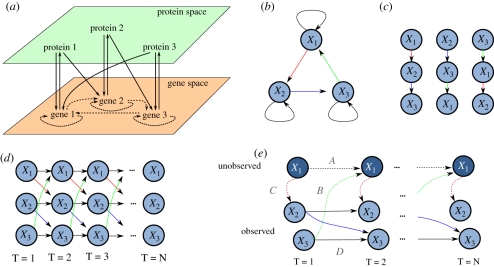
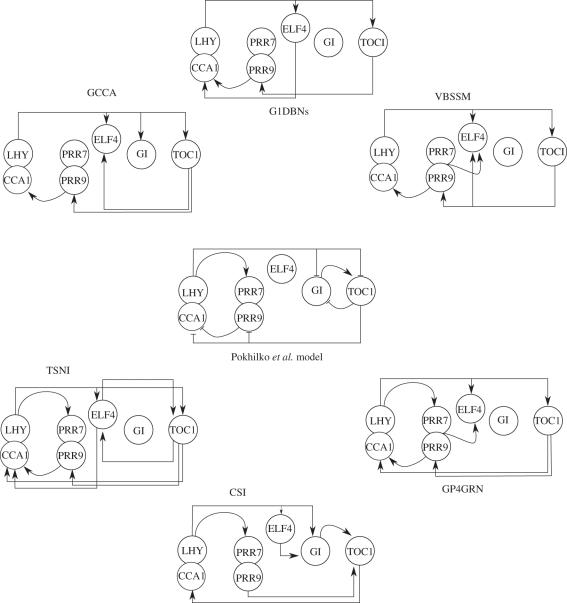
Inferring the topology of a gene-regulatory network (GRN) from genome-scale time-series measurements of transcriptional change has proved useful for disentangling complex biological processes. To address the challenges associated with this inference, a number of competing approaches have previously been used, including examples from information theory, Bayesian and dynamic Bayesian networks (DBNs), and ordinary differential equation (ODE) or stochastic differential equation. The performance of these competing approaches have previously been assessed using a variety of in silico and in vivo datasets. Here, we revisit this work by assessing the performance of more recent network inference algorithms, including a novel non-parametric learning approach based upon nonlinear dynamical systems. For larger GRNs, containing hundreds of genes, these non-parametric approaches more accurately infer network structures than do traditional approaches, but at significant computational cost. For smaller systems, DBNs are competitive with the non-parametric approaches with respect to computational time and accuracy, and both of these approaches appear to be more accurate than Granger causality-based methods and those using simple ODEs models.

Keywords: gene expression; gene-regulatory networks; inference.

Figure 1.

A schematic of a GRN adapted from Brazhnik et al. [1]. The GRN consists of four genes, three of which encode for TFs (genes 1, 3 and 4) and one of which encodes for a protein that catalyses the production of metabolite 2 from metabolite 1. The physical interactions of components at the various levels can be projected into the gene space (dashed lines) to illustrate the complex GRN that we wish to recover.

Figure 2.

(a) An example system composed of three genes that each encode for a TF that regulates two other genes. The GRN to be recovered from time-series data is projected into the gene space as dashed lines. The time-series observations represent the mRNA levels of genes 1, 2 and 3 as X₁, X₂ and X₃, respectively. (b) A graphical representation of the GRN we wish to recover. (c) BNs cannot represent feedback loops, including self-regulation. Consequently, a BN can, at best, only infer one of three linear pathways. (d) A DBN can be unfolded in time to capture the essence of the GRN, including auto-regulation and feedback loops. (e) In some cases, where observations are missing (in this case observation of gene 1) state-space models may be used to capture the influence of the latent profile.

Figure 3.

Illustration of benchmarking recovered GRNs against a known gold standard network. (a) The true gold standard network consists of four genes with three edges, in which genes 1 and 2 both regulate gene 3, which in turn regulates gene 4. (b) The network recovered by inferring the network from time-series data suggests a four gene network in which gene 2 regulates gene 3, with genes 1 and 3 both regulating gene 4. (c) The number of TPs, TNs, FPs or FNs are counted. In this case, the recovered network contains two TPs, one FP, one FN and 12 TNs.

Figure 4.

(a) An example ‘gold standard’ network which consists of four genes with five edges. Gene 1 regulates genes 2 and 3, gene 2 regulates genes 3 and 4 and gene 4 regulates gene 1. (b) The inferred network is a fully connected graph in which particular edges are ranked according to, e.g. the strength or probability of connection. (c) A sparse network can be generated from the fully connected network by removing all edges below a certain threshold. In this example, removing edges below a threshold of 0.1 removes six connections, while a threshold of 0.5 removes nine connections. For threshold the number of TPs, FPs, TNs and FNs can be calculated as in figure 3. A summary of the performance can be obtained using either: (i) the receiver operating characteristic (ROC) curve, which plots 1-FPR versus TPR for all thresholds; or (ii) the precision-recall curve, which plots the TPR versus PPV.

Figure 5.

Inferred networks from the IRMA synthetic yeast network [12] using the switch off dataset. Reconstructed networks consist of the eight top-ranked links inferred by each method. TPs are indicated in solid black lines, with FPs indicated by dashed red lines. Edges that are correct, but have their direction reversed are indicated in dotted red. For the switch off dataset, the CSI algorithm performs best with one incorrect link and one link with reversed direction and one missing link. Networks inferred using knockout data, have only one incorrect link, but with a greater number of links with reversed directions.

Figure 6.

Networks were inferred with the same Arabidopsis thaliana time course data used in Zou et al. [13] and Morrissey et al. [45] on a set of clock genes LHY, CCA1, PRR7, PRR9, TOC1, GI and ELF4 (used in [13]). Networks were identified by taking the top 10 interaction, and subsequently merging LHY with CCA1 and PRR7 with PRR9. For comparison, we include the clock model of Locke et al. [25] and Pokhilko et al. [27]. All algorithms capture the interactions between morning elements LHY/CCA1 and evening elements TOC1/GI and vice versa. Several methods additionally identify the partial loops between LHY/CCA1 and PRR7/PRR9. Most algorithms additionally identify ELF4 as a terminal component of the network.

References

1. Brazhnik P., de la Fuente A., Mendes P. 2002. Gene networks: how to put the function in genomics. Trends Biotechnol. 20, 467–472 10.1016/S0167-7799(02)02053-X (doi:10.1016/S0167-7799(02)02053-X) - DOI - PubMed
1. Park P. J. 2009. ChIP-seq: advantages and challenges of a maturing technology. Nat. Rev. Genet. 10, 669–680 10.1038/nrg2641 (doi:10.1038/nrg2641) - DOI - PMC - PubMed
1. Bulyk M. L. 2005. Discovering DNA regulatory elements with bacteria. Nat. Biotechnol. 23, 942–944 10.1038/nbt0805-942 (doi:10.1038/nbt0805-942) - DOI - PMC - PubMed
1. Berger M. F., Bulyk M. L. 2009. Universal protein-binding microarrays for the comprehensive characterization of the DNA-binding specificities of transcription factors. Nat. Protoc. 4, 393–411 10.1038/nprot.2008.195 (doi:10.1038/nprot.2008.195) - DOI - PMC - PubMed
1. Lopato S., Bazanova N., Morran S., Milligan A. S., Shirley N., Langridge P. 2006. Isolation of plant transcription factors using a modified yeast one-hybrid system. Plant Methods 2, 3. 10.1186/1746-4811-2-3 (doi:10.1186/1746-4811-2-3) - DOI - PMC - PubMed
LinkOut - more resources