The intrinsic connectome of the rat amygdala

Abstract

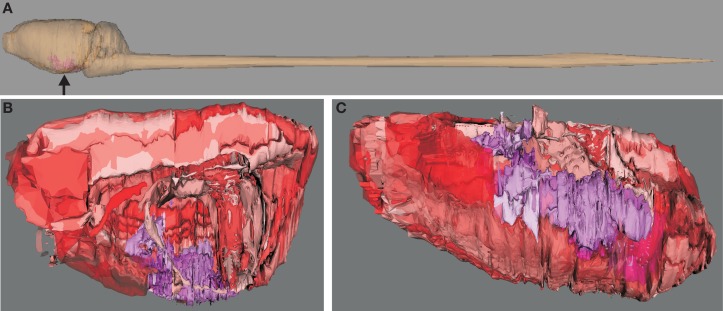
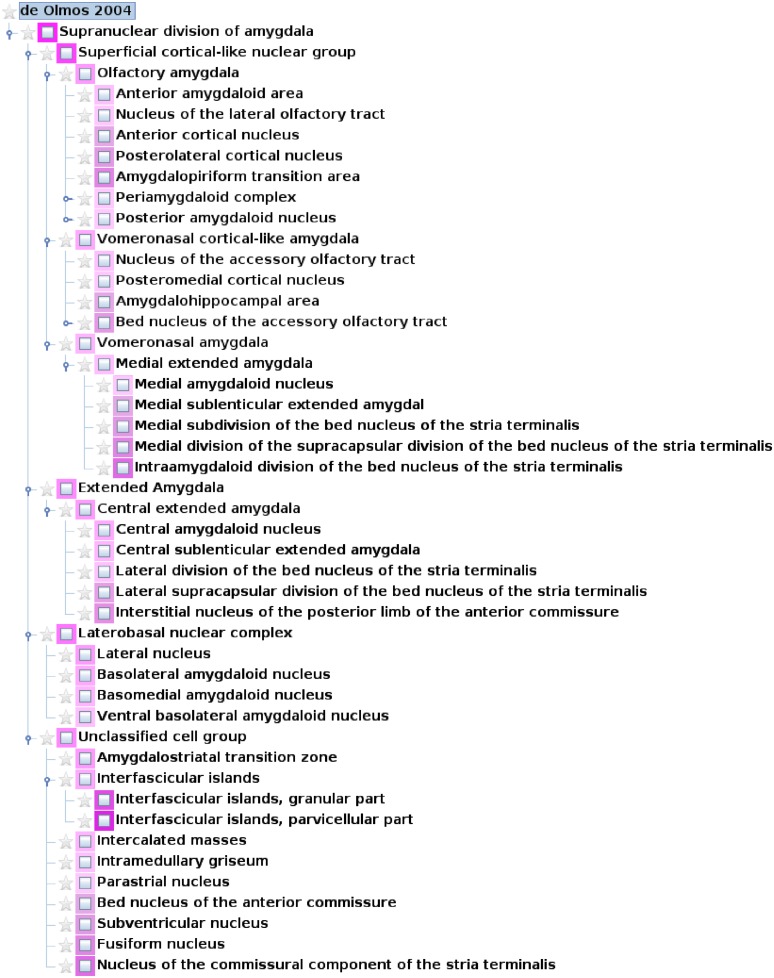
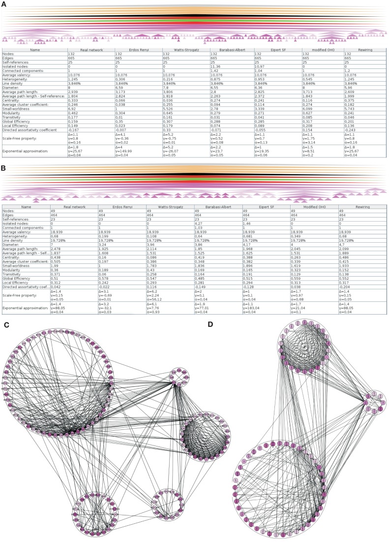
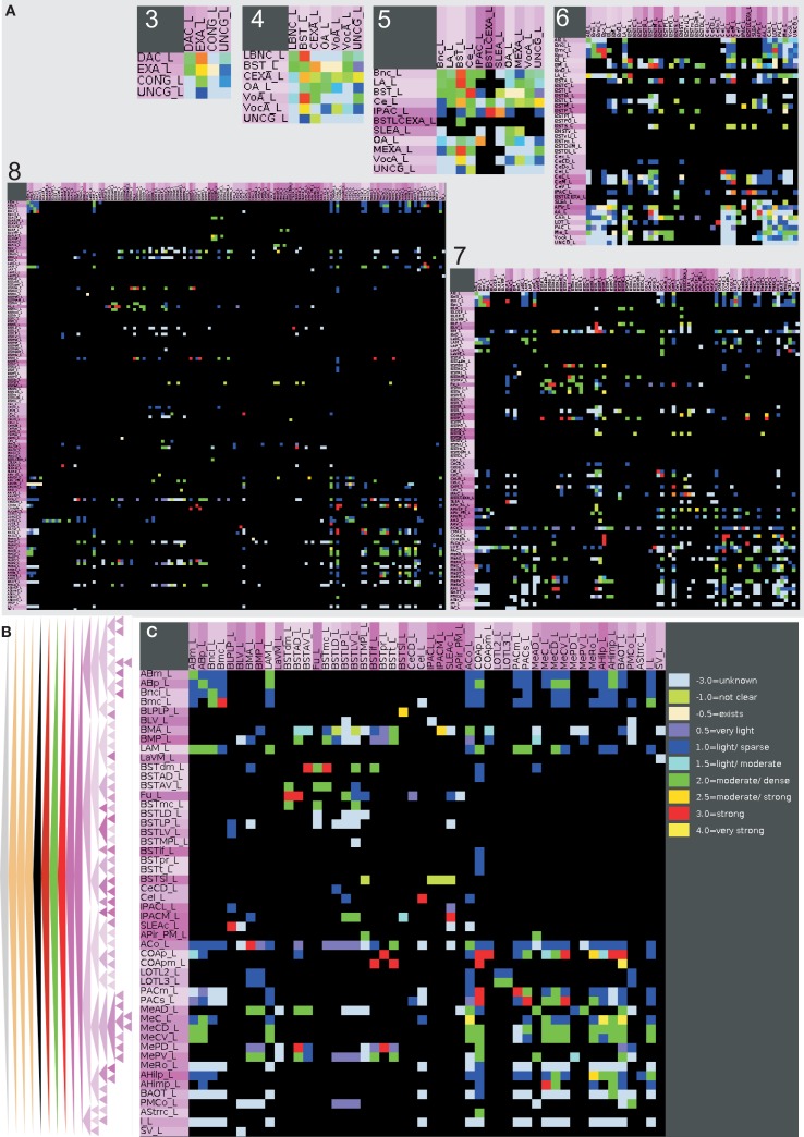
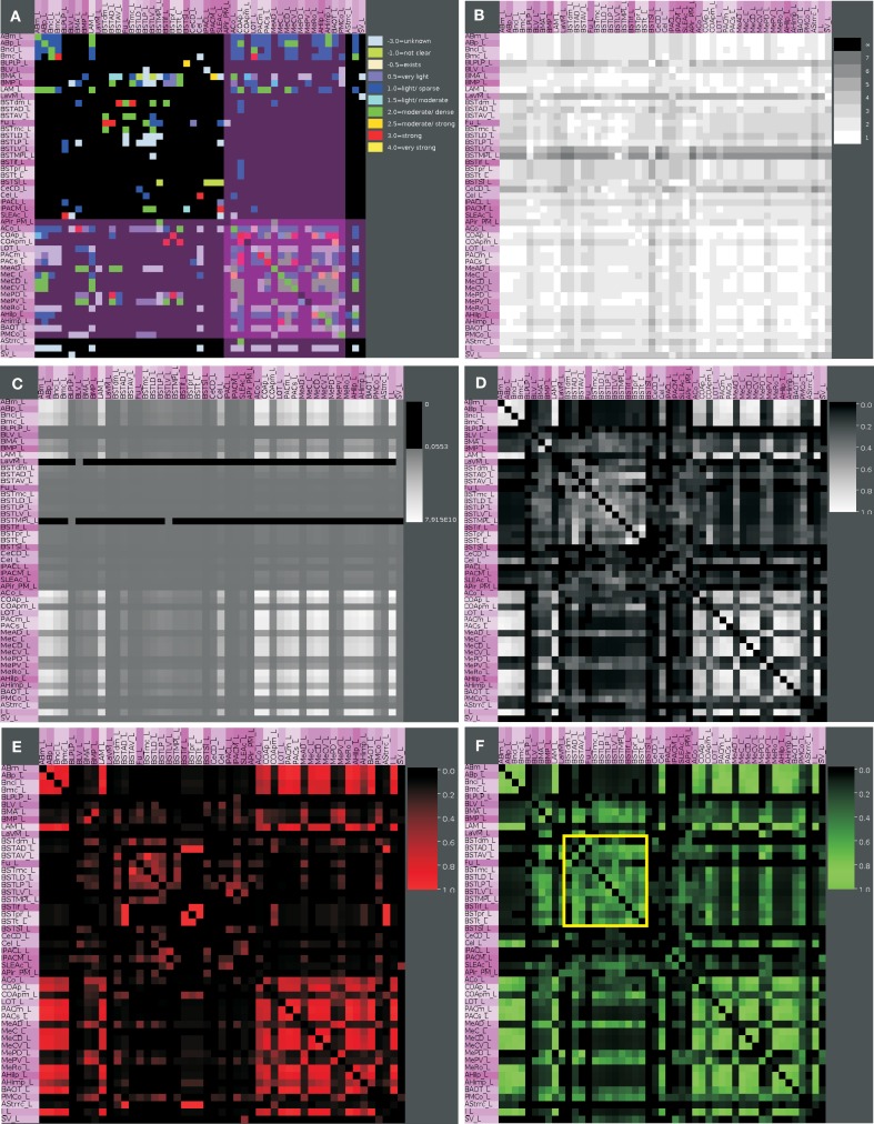
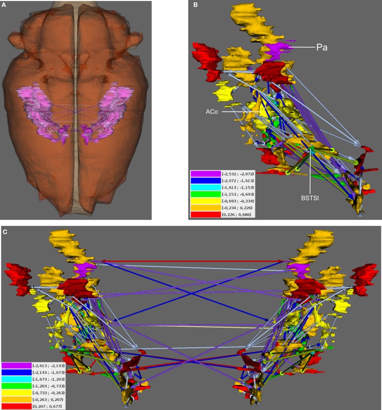
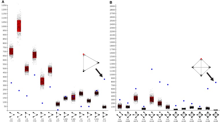
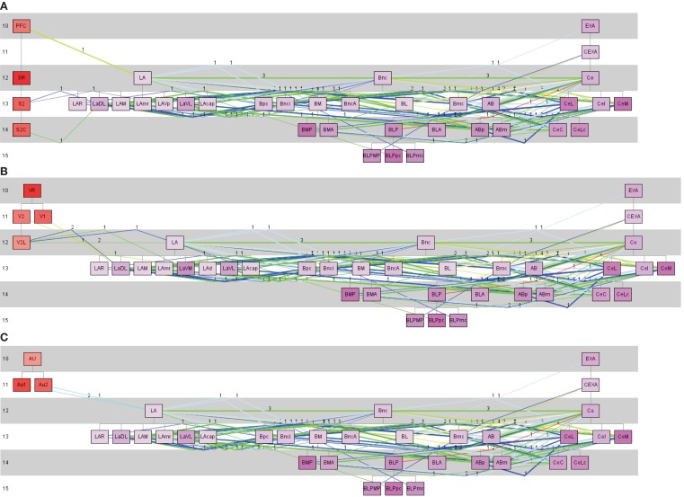
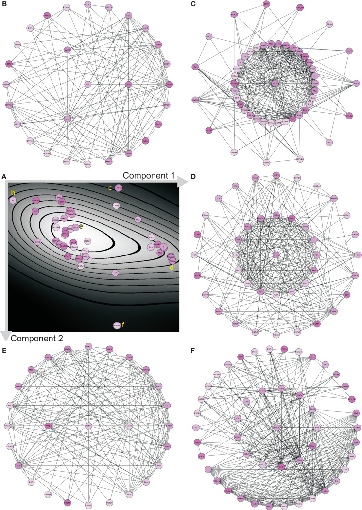
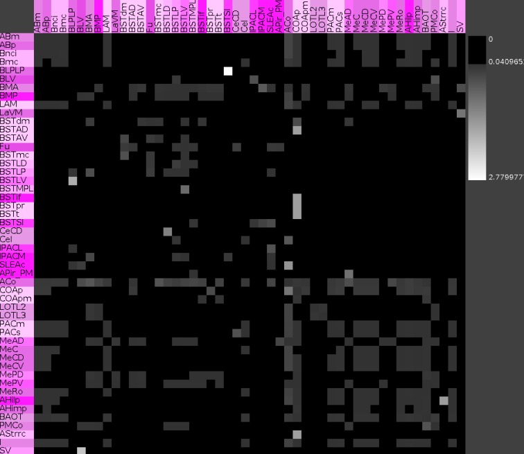
The connectomes of nervous systems or parts there of are becoming important subjects of study as the amount of connectivity data increases. Because most tract-tracing studies are performed on the rat, we conducted a comprehensive analysis of the amygdala connectome of this species resulting in a meta-study. The data were imported into the neuroVIISAS system, where regions of the connectome are organized in a controlled ontology and network analysis can be performed. A weighted digraph represents the bilateral intrinsic (connections of regions of the amygdala) and extrinsic (connections of regions of the amygdala to non-amygdaloid regions) connectome of the amygdala. Its structure as well as its local and global network parameters depend on the arrangement of neuronal entities in the ontology. The intrinsic amygdala connectome is a small-world and scale-free network. The anterior cortical nucleus (72 in- and out-going edges), the posterior nucleus (45), and the anterior basomedial nucleus (44) are the nuclear regions that posses most in- and outdegrees. The posterior nucleus turns out to be the most important nucleus of the intrinsic amygdala network since its Shapley rate is minimal. Within the intrinsic amygdala, regions were determined that are essential for network integrity. These regions are important for behavioral (processing of emotions and motivation) and functional (memory) performances of the amygdala as reported in other studies.

Keywords: amygdala; connectome; network analysis; rat brain; simulation; stereotaxic atlas; tract-tracing; visualization.

Figure 1

Visualization of hierarchical regions of the rat central nervous system using neuroVIISAS. The subdivision of regions of the amygdala is based on the stereotactic atlas of Paxinos and Watson (2007). (A) Location of the amygdala (arrow) in the central nervous system of the rat. (B) The view from the midline into the right hemisphere shows the amygdala (magenta structures). Cortical regions are labeled with red tones [same orientation as shown in (A)]. This scheme of colors is consistent with the color mapping of the complete rat nervous system connectome where further colors are already assigned to other regions (see Materials and Methods). (C) The view from ventral (bottom) shows the rostrocaudal extension of the amygdala. The rough surfaces are caused by the intersection distance, serial sectioning, and small subregions of the amygdala.

Figure 2

A hierarchical nomenclature of subregions of the rat amygdala based on (de Olmos et al., 2004) has been implemented for the rat connectome project in neuroVIISAS. Only the top levels of the hierarchy are shown. Different intensities of magenta indicate different subregions.

Figure 3

Global analysis of the left intrinsic amygdala network applied to (A) all regions (132 regions and 665 edges) and (B) 49 regions that have at least one input and one output that are connected by 464 edges (condensed intrinsic amygdala network). The selected regions of the network are visualized by hierarchies of triangles (top panels). The bottom panels display the global network statistics. Both networks are simulated 1000 times by 6 different network generators and global parameters of 1000 simulations were averaged. The result of a modularity analysis is shown in (C) (all regions) and (D) (regions with at least one input and output). (C) Within the 5 modules the number of connections is larger than in between the modules. (D) The number of modules is reduced to 3 if only those regions are considered that have at least one input and one output (90° rotated view).

Figure 4

Hierarchical connectomes allow the selection of different levels of subdivisions of regions. (A) This multi-level representation is shown in the panel with gray background and applied to the left amygdala with 132 regions from level 3 to level 8. Sources or efferent regions are arranged in rows and target or afferent regions are arranged in columns. The sequence of regions is predefined by the sequence of leafs of the defined region hierarchy (see Materials and Methods). (B) Triangle representation of all regions that have at least one input and one output at level 8 and (C) the corresponding adjacency matrix describing 49 regions and 464 connections.

Figure 5

Connectivity matrices of the condensed intrinsic left amygdala network. (A) Adjacency matrix with highlighted regions (transparent magenta) of the superficial amygdaloid cortex. Ten connectivity weights are color-coded. (B) Distance matrix. Gray levels 1–7 indicate the smallest number of edges between regions. Light gray values indicate short distances. (C) Communicability matrix. The gray scale codes values between 0.0553 and 7.915E10. Large values indicate (e.g., ACo) that many short shortest paths between a pair of regions exist. (D) Connectivity matching matrix for inputs and outputs. The gray level scale is coding values between 0 and 1. Large values indicate similar input and output connections of two regions. (E) Connectivity matching matrix for inputs. Red shades are coding similar inputs of two regions. (F) Connectivity matching matrix for outputs. Green shades are coding the similar outputs of two regions. The yellow square indicates the regions of the bed nucleus of the stria terminalis.

Figure 6

Visualization of Shapley rates in 3D-expansion view of the unilateral and bilateral amygdala. (A) View from dorsal. The left- and right-hemispheric amygdala are visible through the transparent pars cranialis of the central nervous system. (B) Unilateral amygdala with regions that have the lowest Shapley rates (see text) and color-coded weights of connections (color-codes of connections are the same as in Figure 5). Color-coded Shapley rates are assigned to regions. (C) Bilateral amygdala with ipsilateral and contralateral connections.

Figure 7

Motif analysis of the condensed intrinsic amygdala network. Frequency of motifs in the intrinsic amygdala network is indicated by a blue dot. Frequencies of motifs in rewiring randomizations are indicated by black points. Red bars show the standard deviation of motif frequencies. (A) 3-Node directed motif analysis of 13 subgraphs. The abundant fully reciprocal motif (e.g., 3-13, where 3 is the number of nodes of this motif and 13 is the identification number of a this motif) is indicated by an arrow and magnified. (B) 4-Node directed motif analysis. Those subgraphs that were significantly more frequent in the real network are shown.

Figure 8

Pathway analysis of somatosensory, visual and auditory regions of the cerebral cortex and the lateral, basal, and central nuclear complexes of the amygdala. (A) Somatosensory, (B) visual, and (C) auditory cortical regions are defined as source regions of the projection to the lateral (LA) nuclear complex of the amygdala. All subregions of the LA are taken into account as putative target regions. From these LA-target regions connections to the basal nuclear complex (including BL) where searched. From the basal nuclear complex, connections were chosen which project to CE subregions. The colors of lines corresponds to the weight code in Figure 4. Thick lines indicate reciprocal connections and the numbers indicate the number of studies that have documented a particular connection. In the left part are the source regions displayed, then the LA subtree regions are following, then the basal nuclear complex subtree regions, and on the right the subregions of the CE subtree. The numbers at the left part of the pathway-diagrams are indicating hierarchical levels.

Figure 9

PCA analysis of the condensed intrinsic amygdala network. (A) Probability density diagram of the 2-dimensional plane of PCA showing the 49 mapped regions. Component axes are indicated and correspond to Table 5. Yellow letters refer to the circle-diagrams. All circle-diagrams have a center circle that correspond to a region of interest of the PCA-plane in (A). The inner-ring of circles are the 1st neighbors and the outer-ring of circles are the 2nd neighbors of the center region. (B) Subventricular nucleus (SV). (C) Anterior cortical nucleus (ACo). (D) Amygdalohippocampal area medial part (AHimp). (E) Posteromedial cortical nucleus (PMCo). (F) Amygdalostriatal transition area rostrocaudal part.

Figure 10

Vulnerability matrix of the condensed intrinsic amygdala network. Values indicate the decrease of closeness after removing a particular connection. Removal of the connection from the posterior basolateral nucleus lateral part to the supracapsular bed nucleus of the stria terminalis lateral part has the largest significance of 2.78% (lightest gray value).

References

1. Achard S., Bullmore E. (2007). Efficiency and cost of economical brain functional networks. PLoS Comput. Biol. 3:e17.10.1371/journal.pcbi.0030017 - DOI - PMC - PubMed
1. Adolphs R., Tranel D., Damasio H., Damasio A. (1994). Impaired recognition of emotion in facial expressions following bilateral damage to the human amygdala. Nature 372, 669–67210.1038/372669a0 - DOI - PubMed
1. Aggleton J. (2000). “The amygdala – what’s happened in the last decade?” in The Amygdala: A Functional Analysis, ed. Aggleton J. P. (New York: Oxford University Press; ), 2–29
1. Arenas A., Fernández A., Gómez S. (2008). A complex network approach to the determination of functional groups in the neural system of C. elegans. Lect. Notes Comput. Sci. 5151, 9–1810.1007/978-3-540-92191-2_2 - DOI
1. Baltz A., Kliemann L. (2004). “Spectral analysis,” in Network Analysis. Lecture Notes in Computer Science, Vol. 3418, eds Brandes U., Erlebach T. (Berlin: Springer; ), 373–416
LinkOut - more resources