Interplay between distribution of live cells and growth dynamics of solid tumours

Abstract

Experiments show that simple diffusion of nutrients and waste molecules is not sufficient to explain the typical multilayered structure of solid tumours, where an outer rim of proliferating cells surrounds a layer of quiescent but viable cells and a central necrotic region. These experiments challenge models of tumour growth based exclusively on diffusion. Here we propose a model of tumour growth that incorporates the volume dynamics and the distribution of cells within the viable cell rim. The model is suggested by in silico experiments and is validated using in vitro data. The results correlate with in vivo data as well, and the model can be used to support experimental and clinical oncology.

Figure 1

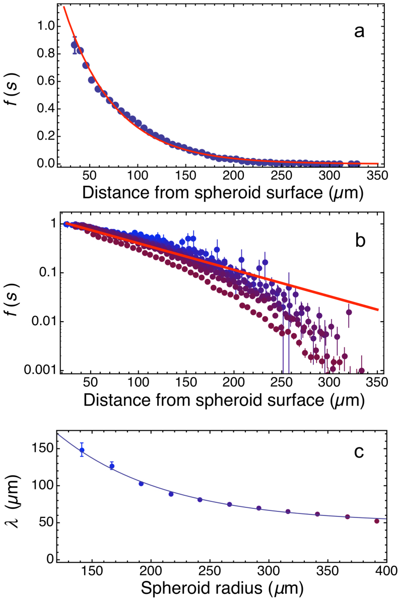
a. Simulation data closely follow the exponential function (4). The plot shows f(s) for a simulated MTS, at about 28.5 days from the start of the numerical experiment with a single initial cell. In this numerical experiment the cell duplication time is about one day. The solid red line is a least-squares exponential regression, which in this case yields λ = 52.7 ± 1.0 μm. b. Simulation data for the same MTS at different times (roughly equally spaced, starting at 12.8 days of simulated time, when about 50% of the cells are still alive near the MTS center; different colors map different times, increasing from blue to dark red) with log vertical scale. In this representation true exponentials should display as straight lines: the straight line is drawn to guide the eye, and corresponds to an exponential with λ = 80 μm. At large depth there is a marked deviation from the exponential behavior, but this is not important in determining the growth law, because the fraction of live cells is very low there, and greater depths also mean spherical shells with smaller volume, which weigh less in the growth law. c. Estimated values of λ from the data in panel b. λ changes slowly as the MTS grows; the solid line is a fit with expression (9).

Figure 2. Total fraction of live cells F(r) estimated from actual experimental data in refs. 17 and 18.

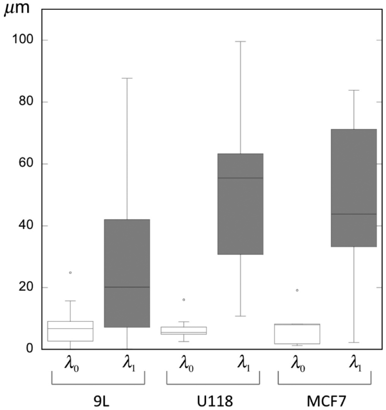
Circles represent the aggregate measurements of individual MTS obtained with Rat1-T1, MR1, and EMT6/Ro cells. The solid black line is the estimate obtained from expression (6), assuming variable λ as defined by equation (9) – Maximum a posteriori (MAP) values are: λ₀ = 48.96 ± 0.05 μm, λ₁ = 77.48 ± 0.05 μm, ζ = 48.96 ± 0.05 μm – while the dashed line is the estimate obtained with constant λ (MAP value: λ_c = 54.64 ± 0.05 μm).

Figure 3. Bayesian analysis of experimental data.

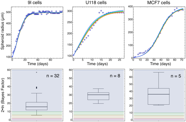
Top panels: representative growth data (circles) of individual tumour MTS obtained with cell lines 9l, U118, and MCF7. The lines show the predictive posteriors computed by Bayesian inference with our model at the following percentile levels: 2.5% (orange), 25% (red), 50% (green), 75% (cyan), 97.5% (blue). Deviation of the data from these model predictions was identified as observation error. Bottom panels: box-plots of the Bayes factor that compares the new model with constant λ and the Gompertz model. The Bayes factors are calculated for n individual MTS, and the box plots represent their distributions. The Bayes factors are always greater than 1 and always favor our model, sometimes strikingly so. The background colored bands show levels of evidence to prefer our model: red, weak evidence; orange, positive evidence; green, strong evidence; blue, very strong evidence (levels are chosen according to the suggestion of Kass and Raftery, see the supplementary text). In this analysis we also obtain Maximum a posteriori (MAP) estimates of the model parameters; we find the following mean values from populations of MAP estimates with constant λ: λ_c = 15.3 ± 1.7 μm (9l); λ_c = 19.3 ± 1.9 μm (U118); λ_c = 16.2 ± 1.9 μm (MCF7).

Figure 4. The box plots summarize the distributions of the MAP estimates of λ_c for the model with constant λ, for the three cell lines.

Figure 5. The box plots summarize the distributions of the MAP estimates of λ₀ and λ₁ for the model with variable λ, for the three cell lines.