Modelling dynamics in protein crystal structures by ensemble refinement

Abstract

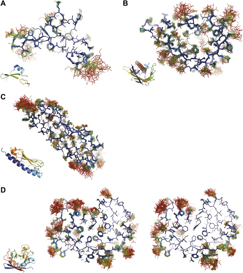
Single-structure models derived from X-ray data do not adequately account for the inherent, functionally important dynamics of protein molecules. We generated ensembles of structures by time-averaged refinement, where local molecular vibrations were sampled by molecular-dynamics (MD) simulation whilst global disorder was partitioned into an underlying overall translation-libration-screw (TLS) model. Modeling of 20 protein datasets at 1.1-3.1 Å resolution reduced cross-validated R(free) values by 0.3-4.9%, indicating that ensemble models fit the X-ray data better than single structures. The ensembles revealed that, while most proteins display a well-ordered core, some proteins exhibit a 'molten core' likely supporting functionally important dynamics in ligand binding, enzyme activity and protomer assembly. Order-disorder changes in HIV protease indicate a mechanism of entropy compensation for ordering the catalytic residues upon ligand binding by disordering specific core residues. Thus, ensemble refinement extracts dynamical details from the X-ray data that allow a more comprehensive understanding of structure-dynamics-function relationships.DOI:http://dx.doi.org/10.7554/eLife.00311.001.

Keywords: None; crystallography; dynamics; function; protein; structure.

Figure 1.

Example of ensemble refinement for dataset 1UOY. (A) Optimisation of empirical ensemble refinement parameters (τ_x, p_TLS and T_bath). Simulations are performed independently and in parallel. The plot shows effect of τ_x, p_TLS on R_free (each grid point corresponds to the lowest R_free among all T_bath values). Optimum parameters are selected by R_free. (B) R-values obtained during ensemble-refinement simulation, solid lines R_work and dashed lines R_free; high values are observed for instantaneous models (yellow) contrasting with the rolling average used in the target function (red) and the final ensemble (blue). (C) R-values are reduced throughout the resolution range for ensemble model (blue) compared with phenix.refine re-refined single structure (black); solid lines R_work and dashed line R_free. (D) Number of structures in the ensemble, reduced by equidistant selection, versus R_work (solid line) and R_free (dashed line). Final number of structures is selected as the minimum number required reproducing the R_free + 0.1%; in this case resulting in an ensemble containing 167 structures. (E) Density difference maps for the ensemble structure (mF_obs − DF_model)exp[iφ_model], left-hand side, and the single structure right-hand side, contoured at 0.34 e/ų (equivalent to 3.0 σ for the ensemble model), positive and negative densities are coloured green and red respectively. All molecular graphics figures are drawn using PyMol (The PyMOL Molecular Graphics System, Schrödinger, LLC). DOI: http://dx.doi.org/10.7554/eLife.00311.004

Figure 2.

Ensemble refinement parameters and results as function of resolution of the datasets. (A) Gain in R_free of ensemble refinement compared with re-refinement using phenix.refine, (B) number of structures in the final ensemble model, (C) optimum relaxation time, τ_x, (D) optimum p_TLS and (E) optimum T_bath plotted as function of resolution of the dataset. DOI: http://dx.doi.org/10.7554/eLife.00311.005

Figure 3.

Validation of ensemble refinement using dataset 1YTT with exceptionally high quality experimental phases. (A) Real space cross-correlation of experimentally phased electron density map (|F_obs|exp[iφ_obs]) and model map (|F_model|exp[iφ_model]) for the single-structure (black) and ensemble model (chain A and B, blue and red respectively) shows improvements particularly for disordered areas (atomic B-factors from the re-refined single structure are shown in grey dashed lines). (B) Example of improved vector-difference map (|F_obs|exp[iφ_obs] − |F_model|exp[iφ_model]), contoured at 0.71 e/ų equivalent to 2.5 σ for the single structure for Gln167, chain A, for single (left-hand side) and ensemble structure (right-hand side). (C) Conformer distribution of Phe121 (chain A) with the experimental phased map (|F_obs|exp[iφ_obs]) contoured at 1.4 σ is highly similar to the multi-conformer shown in Figure 1c in Burling et al. (1996). (D) Partially disordered solvent shell (red) around residue Leu203 (chain A) as anticipated in Burling et al. (1996). Ensemble structure with experimental phased experimental map (|F_obs|exp[iφ_obs]) contoured at 1.4 σ (left side) and 0.7 σ (right side), as shown in Figure 2b in Burling et al. (1996). (E) Scatter plot showing the anti-correlation between the B-factor of explicit solvent molecules in the re-refined single-structure and the relative occupancy of water molecules at that same position (within 0.5-Å distance) in the ensemble model. Due to the difficulty in differentiating between disorder (B-factor) and occupancy for explicitly modelled water atoms in single structures a high B-factor is likely to correspond to a partially occupied site. DOI: http://dx.doi.org/10.7554/eLife.00311.009

Figure 4.

Sampling reproducibility of ensemble refinement. (A) Cross-correlations (CC) calculated for all pairs from 10 random-number seed repeat ensemble refinements of the 1UOY dataset extending to 1.5-Å resolution. (B) Cross correlations computed for 1BV1 (2.0-Å resolution); and, (C) for 3CM8 (2.9-Å resolution). Mean CC shown in solid blue (black error bars indicate ±1 σ). Cross correlations were computed from real-space F_model electron-density map correlations (Brändén and Jones, 1990). B-factors from the single structures refined using phenix.refine are shown in dotted grey lines. DOI: http://dx.doi.org/10.7554/eLife.00311.010

Figure 5.

Reproducibility of side-chain rotamer distributions. Mean χ₁ and χ₂ distributions of four side-chains from the 10 repeats, with error bars ±1 σ, are shown for 1UOY. The four residues presented are those with the two highest CC values (see Figure 4A), (A) Gln11 (0.9999) and (B) Arg32 (0.9999), and the two lowest CC values, (C) Lys39 (0.9976) and (D) Arg13 (0.9966). DOI: http://dx.doi.org/10.7554/eLife.00311.011

Figure 6.

Ramachandran analysis. Distribution of Ramachandran torsion angles classified as outliers (red) and allowed (blue) for ensemble models, 1UOY (A) and 1BV1 (B). Plot shows percentage of classification per residue (i.e. relative number of times a φ,ψ-torsion angle combination is scored as outlier or allowed as defined by phenix.ramalyze). Structure inserts show (left-hand side) the location of the non-favourable torsion angles, outliers (red) and allowed (blue), and (right-hand side) a B-factor putty representation for the single structure refined with phenix.refine. (C) Overall Ramachandran statistics for ensemble and re-refined models. The Ramachandran statistics for the ensemble models are calculated in two ways: blue shows the percentage of outliers (left side) or allowed (right side) from all structures in the ensemble (cf. ‘whole distribution’ in Figure 6—source data 1), whereas red shows these percentages based on the most frequent occurring classification of each φ,ψ combination (cf. ‘centroid distribution’). The grey lines show the percentage of allowed (left side) and outliers (right side) for the re-refined single structures. Ramachandran statistics per re-refined single structure and ensemble are given in Figure 6—source data 2. (D) Correlation of Ramachandran statistics with R_free values obtained from ensemble refinement. Three ensemble refinements were performed for the dataset 1UOY using different random-number seeds at T_bath values of 220, 260, 280, 290 and 295 K. Shown are the number of Ramachandran outliers (left side) and allowed (right side) in the ensemble as function of the R_free value. DOI: http://dx.doi.org/10.7554/eLife.00311.012

Figure 7.

Comparison of atomic fluctuations for non-crystallographic symmetry related protein copies for dataset 1M52. (A) Cα trace of the re-refined single structure coloured by B-factor (from blue to red with increasing B-factor) for the two chains (left) and the B-factors plotted per residue number for protein chain A (blue) and B (red) (right). (B) B-factors from the basal TLS model (left) and rms atomic fluctuations (right) in the ensemble model averaged per residue. Differences in crystal packing restrict the flexibility of chain B around residue 47. (C) Comparison (left) and superposition (right) of a region of the protein (indicated by black box in (A)) of the ensemble of structures observed for protein copy A (blue) and B (red). Analogous analyses for 2R8Q, 1YTT, 1IEP and 2XFA are shown in Figure 7—figure supplements 1–4. The protein copies in 3GWH and 3ODU showed backbone shifts greater than 4.5 Å and were left out of this analysis. DOI: http://dx.doi.org/10.7554/eLife.00311.015

Figure 7—figure supplement 1.

Comparison of atomic fluctuations for NCS related protein copies for dataset 2R8Q. DOI: http://dx.doi.org/10.7554/eLife.00311.016

Figure 7—figure supplement 2.

Comparison of atomic fluctuations for NCS related protein copies for dataset 1YTT. DOI: http://dx.doi.org/10.7554/eLife.00311.017

Figure 7—figure supplement 3.

Comparison of atomic fluctuations for NCS related protein copies for dataset 1IEP. DOI: http://dx.doi.org/10.7554/eLife.00311.018

Figure 7—figure supplement 4.

Comparison of atomic fluctuations for NCS related protein copies for dataset 2XFA. DOI: http://dx.doi.org/10.7554/eLife.00311.019

Figure 8.

Ensemble refinement of two isomorphous proline isomerase datasets collected at 100 K and 288 K. (A) Left, basal TLS B-factors of ensemble models for 100 K and 288 K datasets (blue and green, respectively). Right, atomic rms fluctuations of ensemble models for 100 K and 288 K datasets (blue and green, respectively). (B) Re-refined single-structure (left) and ensemble model (right) for 100 K dataset. (C) Re-refined single-structure and ensemble model for 288 K dataset. In (B) and (C) atoms are coloured by B-factor (5 to 25 Ų). As with the published single structure refinement (Fraser et al., 2009) alternative conformations were not found for residues Leu98, Ser99 and Phe113 at 100K. DOI: http://dx.doi.org/10.7554/eLife.00311.020

Figure 9.

Overview of side-chain dynamics in ensemble structures. Atoms are coloured by their relative probability in the ensemble (see ‘Materials and methods’), reflecting the degree of disorder (ranging from well-ordered in blue to disordered in red). Bottom left insert shows secondary structure cartoon. Three datasets exhibit disordered interior sides chains forming a molten core region. (A) 3CA7 shows an ordered core with disordered hydrophilic side chains on the outside and is typical of the majority of the datasets. (B) 1BV1, the major pollen allergen and putative plant steroid transporter, has a disordered central cavity (location of cavity show with dotted lines). (C) 1X6P in the monomeric form of the fibril forming PAK pilin shows multiple disordered aliphatic and aromatic side chains in the interface between the N-terminal α-helix and the four stranded β-sheet domain. (D) Proline isomerase exhibits a molten core at 288 K, 3K0N (left); however, these interior dynamics are frozen-out at 100 K, 3K0M (right). DOI: http://dx.doi.org/10.7554/eLife.00311.021

Figure 10.

Dynamics in the binding pocket of proline isomerase at 288 K. (A) The location of the binding pocket comprised of residues Arg55, Met61, Ser99 and Phe113. (B) Zoom in of binding pocket (as dotted lines in (A)) showing flexible β-sheet for C=O·HN network of residues 55-62-113-98 in neighbouring β-strands. (C) All four residues show a ∼9:1 ratio between major and minor conformations which is in good agreement with NMR relaxation dispersion data collected a similar temperature (Eisenmesser et al., 2005). Histograms show mean χ₁ angles generated from 10 random number repeats of ensemble refinement (error bars ±1 σ). Inserts show the relevant side chains, coloured by atomic probability (see ‘Materials and methods’), as observed in the ensemble reported in Table 1. DOI: http://dx.doi.org/10.7554/eLife.00311.022

Figure 11.

Comparison of ensemble structures of bound and unbound forms of HIV protease. (A) Residues in the P1 binding sites are disordered in the unbound HIV protease (2PC0), left-hand side, with carbon atoms shown in cyan, oxygen red and nitrogen blue. These residues become ordered in HIV protease in complex with a high affinity inhibitor, JE-2147 (1KZK), right-hand side with carbon atoms of the protease shown in green and of the inhibitor in purple. In 1KZK the two chains of the functional dimer are present in the asymmetric unit, whereas in 2PC0 a monomer is present in the asymmetric unit and the dimer is drawn using the crystallographic twofold axis. (B) Shows an alternative orientation showing the P2 binding site. (C) The catalytic Asp25 becomes ordered upon binding of the inhibitor, forming a hydrogen bond with the P1 carbonyl and hydroxyl of JE-2147. In contrast, the distal residues Cys95 and Leu97 at the dimer interface become less ordered upon binding. DOI: http://dx.doi.org/10.7554/eLife.00311.023

Figure 12.

ABL-kinase Imatinib binding site. (A) Imatinib binding site in chain A of the 1IEP dataset showing distribution of the six protein–ligand hydrogen bonds in chain A and chain B (red and blue respectively). (B) Hydrogen bond network of ordered water network observed in the re-refined single structure, left, and the ensemble model, right. (C) The activation loop (shown in pink) is disordered when ABL-kinase is complexed with Imatinib (shown in cyan) as observed previously in solution (Vajpai et al., 2008). DOI: http://dx.doi.org/10.7554/eLife.00311.024

Figure 13.

Correlation of R-values and overall map correlation coefficient for the 1YTT dataset in the block selection procedure. The correlation coefficients are calculated between the experimentally phased electron density map (|F_obs|exp[iφ_obs]) and ensemble model maps (|F_model|exp[iφ_model]) computed for different blocks of consecutive simulation times; blue squares indicate R_work and red squares indicate R_free. DOI: http://dx.doi.org/10.7554/eLife.00311.026

Figure 14.

Interpretation of global and local details of 1UOY ensemble model is aided by relative atomic probability (as described in ‘Materials and methods’). Ensemble models, left and centre, are colour by individual atom probability (0–1) from red to blue. Single structures, right, are coloured by individual atomic B-factor as refined in phenix.refine. (A) Global structure, selecting different probability ranges highlights partially ordered water positions. (B) Atomic probabilities of loop regain features correlate with B-factors in single structure. Anharmonic motion of Ser5 can be observed as well as anisotropic motion at Tyr7, which is shown in more detail in (C). DOI: http://dx.doi.org/10.7554/eLife.00311.027

References

1. Adams PD, Afonine PV, Bunkóczi G, Chen VB, Davis IW, Echols N, et al. 2010. PHENIX: a comprehensive Python-based system for macromolecular structure solution. Acta Crystallogr D Biol Crystallogr 66:213–21. 10.1107/S0907444909052925 - DOI - PMC - PubMed
1. Adams PD, Pannu NS, Read RJ, Brünger AT. 1997. Cross-validated maximum likelihood enhances crystallographic simulated annealing refinement. Proc Natl Acad Sci USA 94:5018–23 - PMC - PubMed
1. Afonine PV, Grosse-Kunstleve RW, Adams PD. 2005. A robust bulk-solvent correction and anisotropic scaling procedure. Acta Crystallogr D Biol Crystallogr 61:850–5. 10.1107/S0907444905007894 - DOI - PMC - PubMed
1. Afonine PV, Grosse-Kunstleve RW, Echols N, Headd JJ, Moriarty NW, Mustyakimov M, et al. 2012. Towards automated crystallographic structure refinement with phenix.refine. Acta Crystallogr D Biol Crystallogr 68:352–67. 10.1107/S0907444912001308 - DOI - PMC - PubMed
1. Berendsen HJC, Postma JPM, van Gunsteren WF, DiNola A, Haak JR. 1984. Molecular dynamics with coupling to an external bath. The Journal of Chemical Physics 81:3684. 10.1063/1.448118 - DOI
Publication types