. 2012 Dec 20;76(6):1210-24.
doi: 10.1016/j.neuron.2012.10.014.

A continuous semantic space describes the representation of thousands of object and action categories across the human brain

Affiliations

A continuous semantic space describes the representation of thousands of object and action categories across the human brain

Alexander G Huth et al. Neuron. .

Abstract

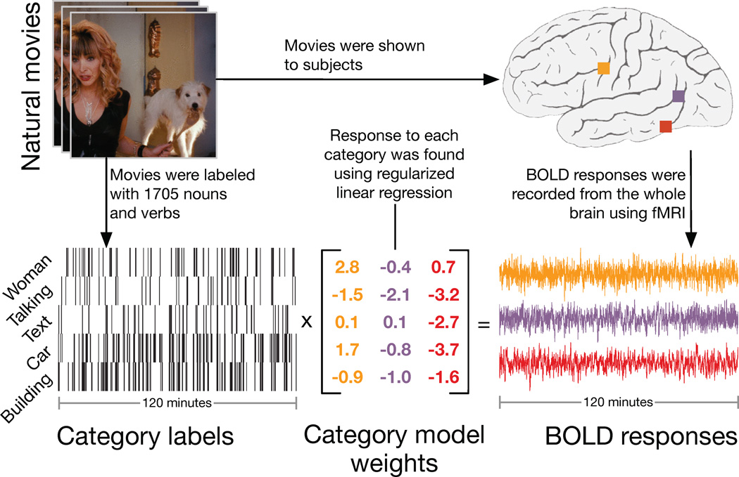
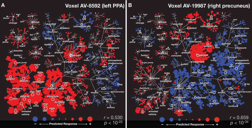
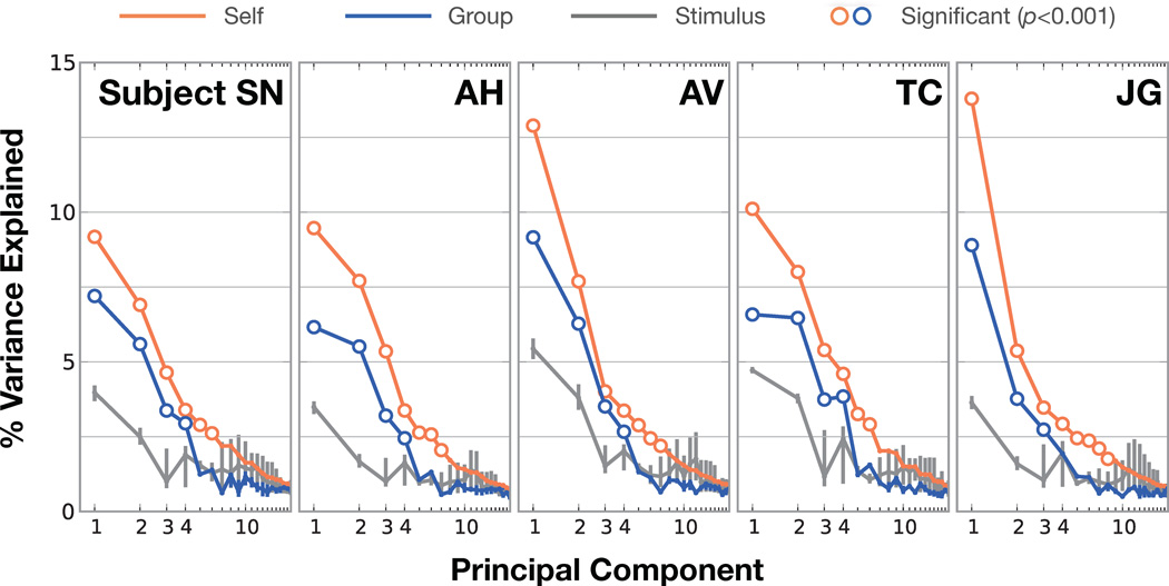
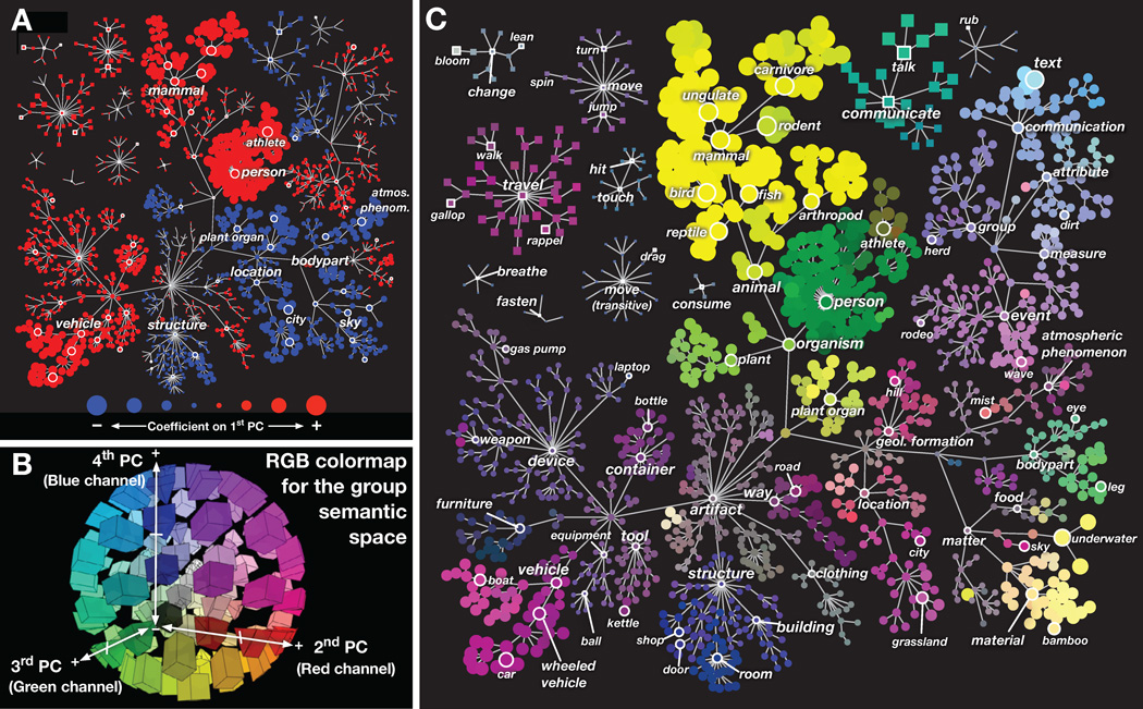
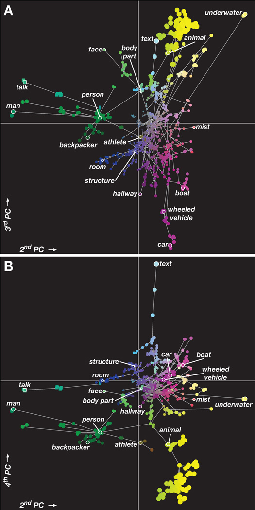
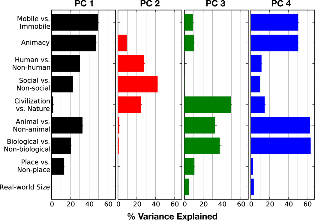
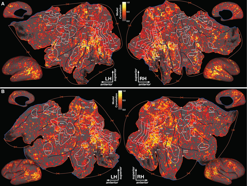
Humans can see and name thousands of distinct object and action categories, so it is unlikely that each category is represented in a distinct brain area. A more efficient scheme would be to represent categories as locations in a continuous semantic space mapped smoothly across the cortical surface. To search for such a space, we used fMRI to measure human brain activity evoked by natural movies. We then used voxelwise models to examine the cortical representation of 1,705 object and action categories. The first few dimensions of the underlying semantic space were recovered from the fit models by principal components analysis. Projection of the recovered semantic space onto cortical flat maps shows that semantic selectivity is organized into smooth gradients that cover much of visual and nonvisual cortex. Furthermore, both the recovered semantic space and the cortical organization of the space are shared across different individuals.


Conflict of interest statement

The authors declare no conflict of interest.

Figures

Figure 1
Figure 1
Schematic of the experiment and model. Subjects viewed two hours of natural movies while BOLD responses were measured using fMRI. Objects and actions in the movies were labeled using 1364 terms from the WordNet lexicon (Miller, 1995). The hierarchical is a relationships defined by WordNet were used to infer the presence of 341 higher- order categories, providing a total of 1705 distinct category labels. A regularized, linearized finite impulse response regression model was then estimated for each cortical voxel recorded in each subject's brain (Kay et al., 2008; Mitchell et al., 2008; Naselaris et al., 2009; Nishimoto et al., 2011). The resulting category model weights describe how various object and action categories influence BOLD signals recorded in each voxel. Categories with positive weights tend to increase BOLD, while those with negative weights tend to decrease BOLD. The response of a voxel to a particular scene is predicted as the sum of the weights for all categories in that scene.
Figure 2
Figure 2
Category selectivity for two individual voxels. Each panel shows the predicted response of one voxel to each of the 1705 categories, organized according to the graphical structure of WordNet. Links indicate is a relationships (e.g. an athlete is a person); some relationships used in the model are omitted for clarity. Each marker represents a single noun (circle) or verb (square). Red markers indicate positive predicted responses and blue negative. The area of each marker indicates predicted response magnitude. The prediction accuracy of each voxel model, computed as the correlation coefficient (r) between predicted and actual responses, is shown in the bottom right of each panel along with model significance (see Results for details). (A) Category selectivity for one voxel located in the left-hemisphere parahippocampal place area (PPA). The category model predicts that movies will evoke positive responses when structures, buildings, roads, containers, devices, and vehicles are present. Thus, this voxel appears to be selective for scenes that contain man-made objects and structures (Epstein & Kanwisher, 1998). (B) Category selectivity for one voxel located in the right-hemisphere precuneus (PrCu). The category model predicts that movies will evoke positive responses from this voxel when people, carnivores, communication verbs, rooms, or vehicles are present, and negative responses when movies contain atmospheric phenomena, locations, buildings, or roads. Thus, this voxel appears to be selective for scenes that contain people or animals interacting socially (Iacoboni et al., 2004).
Figure 3
Figure 3
Amount of model variance explained by individual subject and group semantic spaces. Principal components analysis (PCA) was used to recover a semantic space from category model weights in each subject. Here we show the variance explained in the category model weights by each of the 20 most important PCs. Orange lines show the amount of variance explained in category model weights by each subject's own PCs and blue lines show the variance explained by PCs of combined data from other subjects. Gray lines show the variance explained by the stimulus PCs, which serve as an appropriate null hypothesis (see text and methods for details). Error bars indicate 99% confidence intervals (the confidence intervals for the subjects' own PCs and group PCs are very small). Hollow markers indicate subject or group PCs that explain significantly more variance (p<0.001, bootstrap test) than the stimulus PCs. The first four group PCs explain significantly more variance than the stimulus PCs for four subjects. Thus, the first four group PCs appear to comprise a semantic space that is common across most individuals, and which cannot be explained by stimulus statistics. Furthermore, the first six to nine individual subject PCs explain significantly more variance than the stimulus PCs (p<0.001, bootstrap test). This suggests that while the subjects share broad aspects of semantic representation, finer-scale semantic representations are subject-specific.
Figure 4
Figure 4
Graphical visualization of the group semantic space. (A) Coefficients of all 1705 categories in the first group PC, organized according to the graphical structure of WordNet. Links indicate is a relationships (e.g. an athlete is a person); some relationships used in the model have been omitted for clarity. Each marker represents a single noun (circle) or verb (square). Red markers indicate positive coefficients and blue negative. The area of each marker indicates the magnitude of the coefficient. This PC distinguishes between categories with high stimulus energy (e.g. moving objects like person and vehicle) and those with low stimulus energy (e.g. stationary objects like sky and city). (B) The three-dimensional RGB colormap used to visualize PCs 2–4. The category coefficient in the second PC determined the value of the red channel, the third PC determined the green channel and the fourth PC determined the blue channel. Under this scheme categories that are represented similarly in the brain are assigned similar colors. Categories with zero coefficients appear neutral gray. (C) Coefficients of all 1705 categories in group PCs 2–4, organized according to the WordNet graph. The color of each marker is determined by the RGB colormap in panel B. Marker sizes reflect the magnitude of the three-dimensional coefficient vector for each category. This graph shows that categories thought to be semantically related (e.g. athletes and walking) are represented similarly in the brain.
Figure 5
Figure 5
Spatial visualization of the group semantic space. (A) All 1705 categories, organized by their coefficients on the second and third PCs. Links indicate is a relationships (e.g. an athlete is a person) from the WordNet graph; some relationships used in the model have been omitted for clarity. Each marker represents a single noun (circle) or verb (square). The color of each marker is determined by an RGB colormap based on the category coefficients in PCs 2–4 (see Fig. 4B for details). The position of each marker is also determined by the PC coefficients: position on the x axis is determined by the coefficient on the second PC and position on the y-axis is determined by the coefficient on the third PC. This ensures that categories that are represented similarly in the brain appear near each other. The area of each marker indicates the magnitude of the PC coefficients for that category; more important or strongly represented categories have larger coefficients. The categories man, talk, text, underwater, and car have the largest coefficients on these PCs. (B) All 1705 categories, organized by their coefficients on the second and fourth PCs. Format same as panel A. The large group of animal categories has large PC coefficients, and is mainly distinguished by the fourth PC. Human categories appear to span a continuum. The category person is very close to indoor categories such as room on the second and third PCs, but different on the fourth. The category athlete is close to vehicle categories on the second and third PCs, but is also close to animal on the fourth PC. These semantically-related categories are represented similarly in the brain, supporting the hypothesis of a smooth semantic space. However, these results also show that some categories (e.g. talk, man, text, and car) appear to be more important than others. A movie showing this semantic space in 3D is included in Supplemental Materials.
Figure 6
Figure 6
Comparison between the group semantic space and nine hypothesized semantic dimensions. For each hypothesized semantic dimension we assigned a value to each of the 1705 categories (see methods for details) and we computed the fraction of variance that each dimension explains in each PC. Each panel shows the variance explained by all hypothesized dimensions in one of the four group PCs. Error bars indicate bootstrap standard error. The first PC is best explained by a dimension that contrasts mobile categories (people, non-human animals, and vehicles) with non-mobile categories, and an animacy dimension (Connolly et al, 2012) that assigns high weight to humans, decreasing weights to other mammals, birds, reptiles, fish, and invertebrates and zero weight to other categories. The second PC is best explained by a dimension that contrasts social categories (people and communication verbs) with all other categories. The third PC is best explained by a dimension that contrasts categories associated with civilization (people, man-made objects, and vehicles) with categories associated with nature (non-human animals). The fourth PC is best explained by a dimension that contrasts biological categories (people, animals, plants, body parts, plant parts) with non-biological categories, and a dimension that contrasts animals (people and non-human animals) with non-animals.
Figure 7
Figure 7
Semantic space represented across the cortical surface. (A) The category model weights for each cortical voxel in subject AV are projected onto PCs 2–4 of the group semantic space, and then assigned a color according to the scheme described in Figure 4B. These colors are projected onto a cortical flat map constructed for subject AV. Each location on the flat map shown here represents a single voxel in the brain of subject AV. Locations with similar colors have similar semantic selectivity. This map reveals that the semantic space is represented in broad gradients distributed across much of anterior visual cortex. Semantic selectivity is also apparent in medial and lateral parietal cortex, auditory cortex, and lateral prefrontal cortex. Brain areas identified using conventional functional localizers are outlined in white and labeled (see Table S1 for abbreviations). Boundaries that have been inferred from anatomy or which are otherwise uncertain are denoted by dashed white lines. Major sulci are denoted by dark blue lines and labeled (see Table S2 for abbreviations). Some anatomical regions are labeled in light blue (Abbreviations: PrCu=precuneus; TPJ=temporoparietal junction). Cuts made to the cortical surface during the flattening procedure are indicated by dashed red lines and a red border. The apex of each cut is indicated by a star. Blue borders show the edge of the corpus callosum and sub-cortical structures. Regions of fMRI signal dropout due to field inhomogeneity are shaded with black hatched lines. (B) Projection of voxel model weights onto the first PC for subject AV. Voxels with positive projections on the first PC appear red, while those with negative projections appear blue and those orthogonal to the first PC appear gray. (C) Projection of voxel weights onto PCs 2–4 of the group semantic space for subject TC. (D) Projection of voxel model weights onto the first PC for subject TC. See Figure S5 for maps of semantic representation in other subjects. Note: Explore these datasets yourself at http://gallantlab.org/semanticmovies
Figure 8
Figure 8
Smoothness of cortical maps under the group semantic space. To quantify smoothness of cortical representation under a semantic space, we first projected voxel category model weights into the semantic space. Then we computed the mean correlation between voxel semantic projections as a function of the distance between voxels along the cortical sheet. To determine whether cortical semantic maps under the group semantic model are significantly smoother than chance, smoothness was computed using the same analysis for 1000 random 4-dimensional spaces. Mean correlations for the group semantic space are plotted in blue, and mean correlations for the 1000 random spaces are plotted in gray. Gray error bars show 99% confidence intervals for the random space results. Group semantic space correlations that are significantly different from the random space results (p<0.001) are shown as hollow symbols. For adjacent voxels (distance 1) and voxels separated by one intermediate voxel (distance 2), correlations of group semantic space projections are significantly greater than chance in all subjects. This shows that cortical semantic maps under the group semantic space are much smoother than would be expected by chance.
Figure 9
Figure 9
Model prediction performance across the cortical surface. To determine how much of the response variance of each voxel is explained by the category model, prediction performance was assessed using separate validation data reserved for this purpose. (A) Each location on the flat map represents a single voxel in the brain of subject AV. Colors reflect prediction performance on the validation data. Well predicted voxels appear yellow or white, and poorly predicted voxels appear gray. The best predictions are found in occipitotemporal cortex, the posterior superior temporal sulcus, medial parietal cortex, and inferior frontal cortex. (B) Model performance for subject TC. See Figure S7 for model prediction performance in other subjects. See Table S3 for model prediction performance within known functional areas.

References

    1. Adelson EH, Bergen JR. Spatiotemporal energy models for the perception of motion. J Opt Soc Am A. 1985;2(2):284–299. - PubMed
    1. Aguirre GK, Zarahn E, D’esposito M. An Area within Human Ventral Cortex Sensitive to Building Stimuli: Evidence and Implications. Neuron. 1998;21(2):373–383. - PubMed
    1. Avidan, Hasson U, Malach R, Behrmann M. Detailed exploration of face-related processing in congenital prosopagnosia 2. Functional neuroimaging findings. J Cogn Neurosci. 2005;17(7):1150–1167. - PubMed
    1. Bartels A, Zeki S. Functional brain mapping during free viewing of natural scenes. Hum Brain Mapp. 2004;21(2):75–85. - PMC - PubMed
    1. Buccino G, Binkofski F, Fink GR, Fadiga L, Fogassi L, Gallese V, Seitz RJ, et al. Action observation activates premotor and parietal areas in a somatotopic manner: an fMRI study. Eur J Neurosci. 2001;13(2):400. - PubMed

Publication types