Source reconstruction accuracy of MEG and EEG Bayesian inversion approaches

Abstract

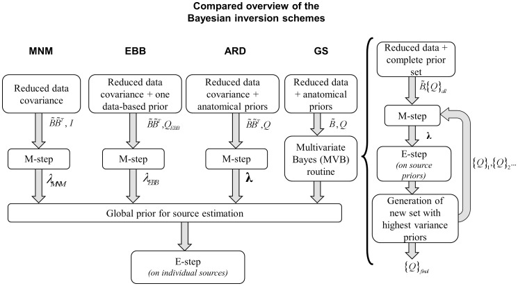
Electro- and magnetoencephalography allow for non-invasive investigation of human brain activation and corresponding networks with high temporal resolution. Still, no correct network detection is possible without reliable source localization. In this paper, we examine four different source localization schemes under a common Variational Bayesian framework. A Bayesian approach to the Minimum Norm Model (MNM), an Empirical Bayesian Beamformer (EBB) and two iterative Bayesian schemes (Automatic Relevance Determination (ARD) and Greedy Search (GS)) are quantitatively compared. While EBB and MNM each use a single empirical prior, ARD and GS employ a library of anatomical priors that define possible source configurations. The localization performance was investigated as a function of (i) the number of sources (one vs. two vs. three), (ii) the signal to noise ratio (SNR; 5 levels) and (iii) the temporal correlation of source time courses (for the cases of two or three sources). We also tested whether the use of additional bilateral priors specifying source covariance for ARD and GS algorithms improved performance. Our results show that MNM proves effective only with single source configurations. EBB shows a spatial accuracy of few millimeters with high SNRs and low correlation between sources. In contrast, ARD and GS are more robust to noise and less affected by temporal correlations between sources. However, the spatial accuracy of ARD and GS is generally limited to the order of one centimeter. We found that the use of correlated covariance priors made no difference to ARD/GS performance.

Figure 1. The four common stages for the algorithm comparison.

1. Data preprocessing (common to all schemes) 2. Prior definition (multiple (ARD and GS) or single (MNM AND EBB)) 3. Prior weighting through ReML 4. Source localization (again, common to the four schemes).

Figure 2. Profile intensities G(s) of the same spatial pattern for different values of the smoothness parameter s.

LEFT: the location and maximum extent of the spatial pattern is shown (blue region). RIGHT: the spatial pattern is shown for different s values ranging from 0.2 to 0.8, projected on the cortical surface (left) and on a flattened surface upon a wireframe height map (right). The number of points featuring more than 60% of the G peak value (central point of the spatial pattern) can range from 20 (s = 0.2) to 55 (s = 0.8).

Figure 3. Overview of the four schemes pipeline.

In the MNM and EBB case the M-step just provides a scaling factor on its single prior, while ARD uses it to weight and select source priors which give a relevant contribution. GS handles proposed sets of priors, discarding the irrelevant ones (applying the M-step), and introducing a new set with the most active priors (as estimated by the internal E-step). Finally, the common E-step at the end is the only stage where individual sources are evaluated.

Figure 4. Possible simulated source locations.

External and internal views of the brain hemispheres are shown in the upper and lower part of the image respectively. The algorithm for the source site choice aims to minimize the spatial pattern overlap.

Figure 5. Synthetic time courses for one simulation.

For each source, a frequency per time sample is drawn from a Gaussian distribution , top row). The instantaneous source amplitude is obtained by integrating the frequencies and taking the sine of the resulting angle. If the generated time course satisfies the desired correlation threshold (either high or low: middle and lower rows, respectively), it is accepted; otherwise the procedure is repeated. The corresponding frequency histogram and correlation matrices are shown in the right column.

Figure 6. Example of localization performances at 0 and 20 dB.

Two asymmetrical, weakly correlated sources are simulated in the forward problem. Symmetrical correlated priors are considered for ARD and GS. The actual simulated dipoles are centered at the dashed circles. EBB performs almost flawlessly at high SNR at high SNR. GS and ARD still show some local maxima in the actual source location at extremely low SNR.

Figure 7. Example of a Positive Predictive Value (PPV) curve for one simulation’s source localization, calculated by means of the localization image volume.

The PPV is the proportion of the images peaks that are localized within a given search-size around the simulated dipole (True Positives, TP). Peaks localized outside of the search-size are considered False Positives (FP). Thus, PPV is TP/(TP+FP). The peaks are ordered by intensity, and PPV is calculated for each fraction of the total peak count. In this way, a curve is obtained that indicates whether the stronger peaks fall near the dipole (decreasing slope) or far from it (increasing slope). The area under the curve was used as a performance indicator, the Spatial Accuracy Index (SAI). The curves in the figure depict 10 search-sizes from 3 to 30 mm, on a logarithmic scale.

Figure 8. Example of curves of temporal variance explained by the source reconstruction (R²).

The R² value reported by SPM includes all vertices in the cortical mesh. Only the vertices located within the given search-size (x axis; 3 to 30 mm) were considered to generate time-courses. One line plot is calculated for each SNR (−30 to +10 dB, in 10 dB steps). The Temporal Accuracy Index (TAI) for a given search-size is considered as the R² value at that distance.

Figure 9. Summary of spatial (SAI) and temporal (TAI) accuracies of the four algorithms. A: Magnified example of a scale value grid for explanatory purposes.

The color coded values represent the areas under the curve (AUC) pertaining to the spatial and temporal accuracy curves. AUC values are plotted as functions of SNR (x axis, −30 dB to 10 dB) and search-size (y axis, 3 mm to 30 mm, downward direction, logarithmic scale). B, C: Spatial (B) and temporal (C) accuracies were evaluated for 1, 2 and 3 dipoles. Different conditions were manipulated: (1) Symmetry of 2 sources (symmetric vs. asymmetric in the two hemispheres); (2) Correlation level between sources (high or low, for 2 and 3 sources); (3) Bilateral correlated source priors vs absence of them (only ARD and GS). ‘bi’ stands for correlated priors included. ‘uni’ stands for correlated priors omitted.

Figure 10. Statistical comparison of the inversion schemes for a search-size of 14 mm.

ARD (green), GS (red), EBB (blue) and MNM results are plotted in Panel A (SAI results) and B (TAI results). For each simulation the mean accuracy index is plotted versus the different SNR levels. The error bars show the standard error. Black squares in the lower panels indicate significant difference between the schemes’ performances.

Figure 11. Statistical validation of performances under conditions of high correlation.

Upper panel: Plots of ARD and GS performances with highly correlated symmetrical sources in case of inclusion (green) or exclusion of symmetric source priors (black). Lower panel: Differences between EBB performances with high (black) and low (green) correlated sources. The black squares represent significant differences in correspondence of the different SNRs.

References

1. Liljeström M, Kujala J, Jensen O, Salmelin R (2005) Neuromagnetic localization of rhythmic activity in the human brain: a comparison of three methods. NeuroImage 25: 734–745. - PubMed
1. Schoffelen J, Gross J (2009) Source connectivity analysis with MEG and EEG. Human Brain Mapping 30: 1857–1865. - PMC - PubMed
1. Sekihara K, Sahani M, Nagarajan S (2005) Localization bias and spatial resolution of adaptive and non-adaptive spatial filters for MEG source reconstruction. NeuroImage 25: 1056–1067. - PMC - PubMed
1. Wipf D, Nagarajan S (2009) A unified Bayesian framework for MEG/EEG source imaging. NeuroImage 44 947–966. - PMC - PubMed
1. Baillet S, Mosher JC, Leahy RM (2001) Electromagnetic brain mapping. IEEE Signal processing magazine 18: 14–30.
Publication types