Modeling the winter-to-summer transition of prokaryotic and viral abundance in the Arctic Ocean

Abstract

One of the challenges in oceanography is to understand the influence of environmental factors on the abundances of prokaryotes and viruses. Generally, conventional statistical methods resolve trends well, but more complex relationships are difficult to explore. In such cases, Artificial Neural Networks (ANNs) offer an alternative way for data analysis. Here, we developed ANN-based models of prokaryotic and viral abundances in the Arctic Ocean. The models were used to identify the best predictors for prokaryotic and viral abundances including cytometrically-distinguishable populations of prokaryotes (high and low nucleic acid cells) and viruses (high- and low-fluorescent viruses) among salinity, temperature, depth, day length, and the concentration of Chlorophyll-a. The best performing ANNs to model the abundances of high and low nucleic acid cells used temperature and Chl-a as input parameters, while the abundances of high- and low-fluorescent viruses used depth, Chl-a, and day length as input parameters. Decreasing viral abundance with increasing depth and decreasing system productivity was captured well by the ANNs. Despite identifying the same predictors for the two populations of prokaryotes and viruses, respectively, the structure of the best performing ANNs differed between high and low nucleic acid cells and between high- and low-fluorescent viruses. Also, the two prokaryotic and viral groups responded differently to changes in the predictor parameters; hence, the cytometric distinction between these populations is ecologically relevant. The models imply that temperature is the main factor explaining most of the variation in the abundances of high nucleic acid cells and total prokaryotes and that the mechanisms governing the reaction to changes in the environment are distinctly different among the prokaryotic and viral populations.

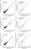
Figure 1. Linear least-squares regression analyses of observed versus predicted prokaryotic abundance.

The figure shows the results of the linear least-squares regression analysis computed for the training and test data sets for the abundances of (A) HNA, (C) LNA, and (E) total prokaryotic abundance (r ² = 0.898; y = 0.456+0.896 x). Additionally, the results of the spatial data set (region designations as in [20]) used for evaluating the trained ANNs are shown for the abundances of (B) HNA, (D) LNA, and (F) total prokaryotic abundance (r ² = 0.703; y = 0.621+1.107 x). Solid lines represent the linear least-squares fit to the data and dashed lines the theoretical 1∶1 fit. The parameters for the linear least-squares regression analyses for panels A–D can be found in Table 3.

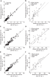
Figure 2. Linear least-squares regression analysis of observed versus predicted viral abundances.

The figure shows the results of the linear least-squares regression analysis computed for the training and test data set of the abundances of (A) V1 viruses, (C) V2 viruses, and (E) total viral abundance (r ² = 0.929; y = 0.425+0.934 x). Additionally, the results of the spatial data set (region designations as in [20]) used for evaluating the trained ANNs are shown for the abundances of (B) V1 viruses, (D) V2 viruses, and (F) total viral abundance (r ² = 0.599; y = 3.495+0.897 x). Solid lines represent the linear least-squares fit to the data and dashed lines the theoretical 1∶1 fit. The parameters for the linear least-squares regression analyses can be found in Table 3.

Figure 3. Data frequency distribution.

The figure shows the frequency distribution of the seasonal data (comprised of the training and test data) over the parameter space used in the ANN-based simulations. The distributions for (A) temperature and Chl-a, (B) day length and Chl-a, and (C) depth are shown.

Figure 4. Simulation of prokaryotic abundance.

The figure shows the abundances of (A) HNA, (B) LNA, and (C) total prokaryotic abundance. The ANNs described in Table 3 were used to simulate the abundances of HNA and LNA cells at temperatures ranging from −1.8–2.8°C and Chl-a ranging from 0.01–0.61 µg L⁻¹. Total prokaryotic abundance was computed by summing the simulated abundances of HNA and LNA cells.

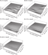
Figure 5. Simulation of the abundance of V1 viruses.

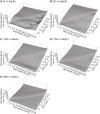
The figure shows the abundance of V1 viruses at a depth of (A) 5 m, (B) 50 m, (C) 100 m, (D) 150 m, and (E) 200 m. The ANN described in Table 3 was used to simulate the abundance of V1 viruses at day lengths ranging from 0–24 hours and Chl-a from 0.01–0.61 µg L⁻¹.

Figure 6. Simulation of the abundance of V2 viruses.

The figure shows the abundance of V2 viruses at a depth of (A) 5 m, (B) 50 m, (C) 100 m, (D) 150 m, and (E) 200 m. The ANN described in Table 3 was used to simulate the abundance of V2 viruses at day lengths ranging from 0–24 hours and Chl-a from 0.01–0.61 µg L⁻¹.

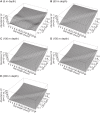
Figure 7. Simulation of viral abundance.

The figure shows total viral abundance at a depth of (A) 5 m, (B) 50 m, (C) 100 m, (D) 150 m, and (E) 200 m. The ANNs described in Table 3 were used to simulate the abundances of V1 and V2 viruses at day lengths ranging from 0–24 hours and Chl-a from 0.01–0.61 µg L⁻¹. Total viral abundance was computed by summing the simulated abundances of V1 and V2 viruses.

References

1. Carmack EC, MacDonald RW (2002) Oceanography of the Canadian shelf of the Beaufort Sea; a setting for marine life. Arctic 55: 29–45.
1. Stein R, Macdonald RW (2004) The organic carbon cycle in the Arctic Ocean. Springer Verlag. 364 p.
1. Yamamoto-Kawai M, Carmack E, McLaughlin F (2006) Nitrogen balance and Arctic throughflow. Nature 443: 43. - PubMed
1. Peterson BJ, McClelland J, Curry R, Holmes RM, Walsh JE, et al. (2006) Trajectory shifts in the arctic and subarctic freshwater cycle. Science 313: 1061–1066. - PubMed
1. Shimada K, Kamoshida T, Itoh M, Nishino S, Carmack E, et al. (2006) Pacific Ocean inflow: influence on catastrophic reduction of sea ice cover in the Arctic Ocean. Geophys Res Lett 33: L08605.
Publication types