

Prey patch patterns predict habitat use by top marine predators with diverse foraging strategies
- PMID: 23301063
- PMCID: PMC3536749
- DOI: 10.1371/journal.pone.0053348
Prey patch patterns predict habitat use by top marine predators with diverse foraging strategies
Abstract
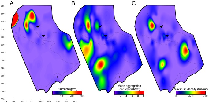
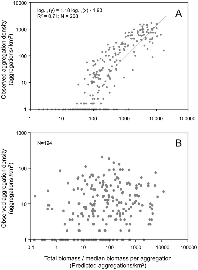
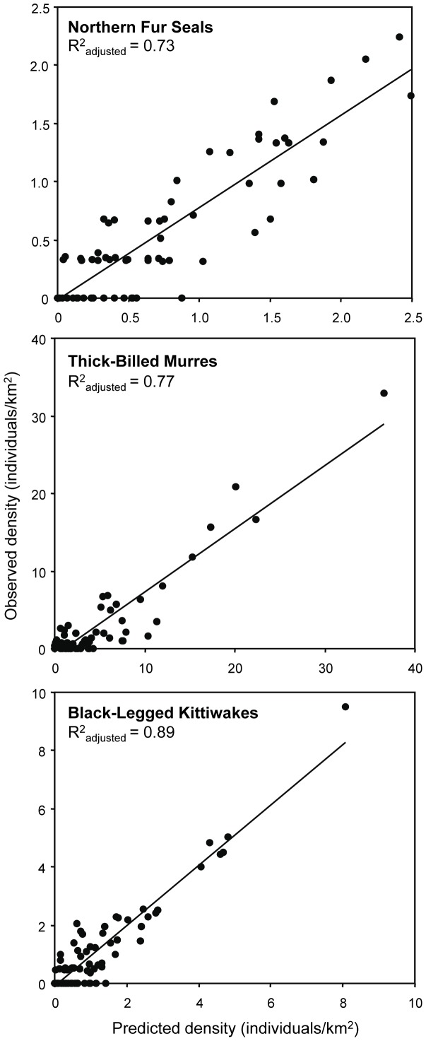
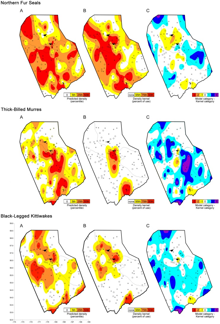
Spatial coherence between predators and prey has rarely been observed in pelagic marine ecosystems. We used measures of the environment, prey abundance, prey quality, and prey distribution to explain the observed distributions of three co-occurring predator species breeding on islands in the southeastern Bering Sea: black-legged kittiwakes (Rissa tridactyla), thick-billed murres (Uria lomvia), and northern fur seals (Callorhinus ursinus). Predictions of statistical models were tested using movement patterns obtained from satellite-tracked individual animals. With the most commonly used measures to quantify prey distributions--areal biomass, density, and numerical abundance--we were unable to find a spatial relationship between predators and their prey. We instead found that habitat use by all three predators was predicted most strongly by prey patch characteristics such as depth and local density within spatial aggregations. Additional prey patch characteristics and physical habitat also contributed significantly to characterizing predator patterns. Our results indicate that the small-scale prey patch characteristics are critical to how predators perceive the quality of their food supply and the mechanisms they use to exploit it, regardless of time of day, sampling year, or source colony. The three focal predator species had different constraints and employed different foraging strategies--a shallow diver that makes trips of moderate distance (kittiwakes), a deep diver that makes trip of short distances (murres), and a deep diver that makes extensive trips (fur seals). However, all three were similarly linked by patchiness of prey rather than by the distribution of overall biomass. This supports the hypothesis that patchiness may be critical for understanding predator-prey relationships in pelagic marine systems more generally.
Conflict of interest statement
Figures
References
-
- Krebs JR (1978) Optimal foraging: Decision rules for predators. In: Krebs JR, Davies NB, editors. Behavioural Ecology, an Evolutionary Approach. Sunderland, MA: Sinauer. 23–63.
-
- Fretwell SD, Lucas HL (1970) On territorial behaviour and other factors influencing habitat distribution in birds. I. Theoretical development. Acta Biotheor 19: 16–36.
-
- Barnett A, Semmens JM (2012) Sequential movement into coastal habitats and high spatial overlap of predator and prey suggest high predation pressure in protected areas. Oikos 121: 882–890.
-
- Wirsing AJ, Cameron KE, Heithaus MR (2010) Spatial responses to predators vary with prey escape mode. Anim Behav 79: 531–537.
-
- Lima SL (2002) Putting predators back into behavioral predator-prey interactions. Trends Ecol Evol 17: 70–75.
Publication types
MeSH terms
LinkOut - more resources
Full Text Sources
Other Literature Sources
