Peak and persistent excess of genetic diversity following an abrupt migration increase

Abstract

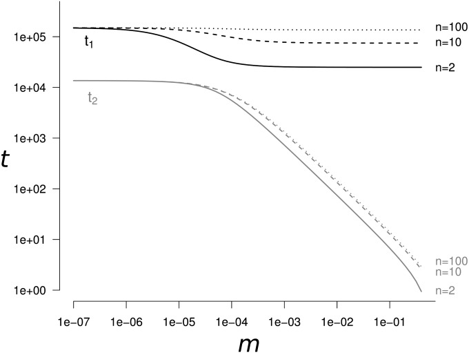
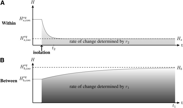
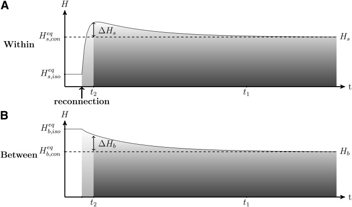
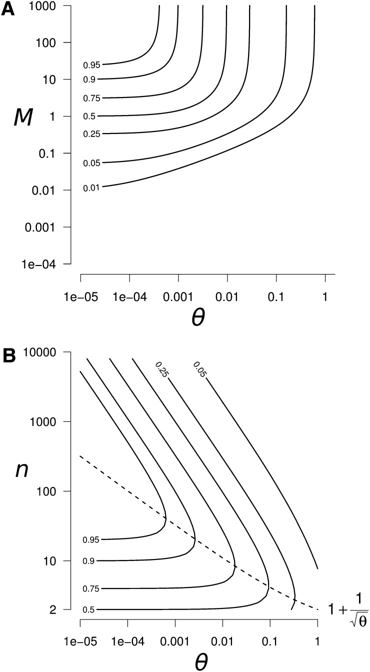
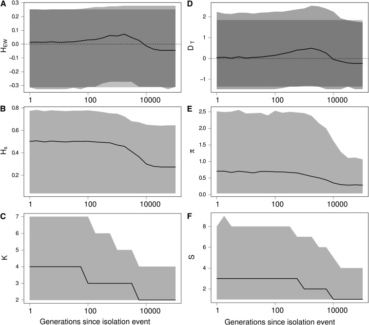
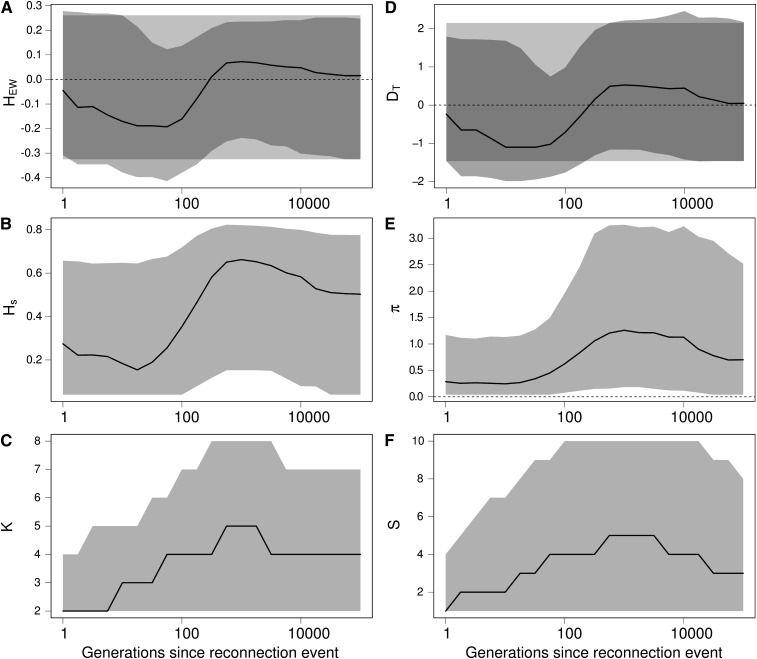
Genetic diversity is essential for population survival and adaptation to changing environments. Demographic processes (e.g., bottleneck and expansion) and spatial structure (e.g., migration, number, and size of populations) are known to shape the patterns of the genetic diversity of populations. However, the impact of temporal changes in migration on genetic diversity has seldom been considered, although such events might be the norm. Indeed, during the millions of years of a species' lifetime, repeated isolation and reconnection of populations occur. Geological and climatic events alternately isolate and reconnect habitats. We analytically document the dynamics of genetic diversity after an abrupt change in migration given the mutation rate and the number and sizes of the populations. We demonstrate that during transient dynamics, genetic diversity can reach unexpectedly high values that can be maintained over thousands of generations. We discuss the consequences of such processes for the evolution of species based on standing genetic variation and how they can affect the reconstruction of a population's demographic and evolutionary history from genetic data. Our results also provide guidelines for the use of genetic data for the conservation of natural populations.

Figure 1

The time (in number of generations) t₁ to reach genetic diversity equilibrium and the length of the transient dynamics period t₂ as a function of the migration rate m. The solid line corresponds to n = 2 populations, the dashed line to n = 10, and the dotted line to n = 100. t₁ is always at least one order of magnitude higher than t₂. This separation of the two periods becomes even greater when $m>1/4N={10}^{-4}$. Parameter values are N = 2500, μ = 10⁻⁵, α = 5%.

Figure 2

Dynamics of (A) within-population H_s and (B) between-population H_b genetic diversity after an isolation event. Within- and between-population diversity (solid lines) were previously at their respective connection equilibrium $H_{\text{s,con}}^{\text{eq}}$ and $H_{\text{b,con}}^{\text{eq}}$. After the isolation event, within- and between-population diversities reach their isolation equilibrium $H_{\text{s,iso}}^{\text{eq}}$ and $H_{\text{b,iso}}^{\text{eq}}$ (dashed lines) at rates determined by r₂ and r₁ (Equation 6). t₂ and t₁ estimate the time to reach the within- and between-population genetic diversity equilibrium, respectively (Equation 8). Under the effect of genetic drift, within-population diversity reaches its equilibrium value faster than between-population genetic diversity. Parameters are n = 10, N = 2500, m = 10⁻⁴ before isolation and m = 0 afterward, and μ = 10⁻⁵. t₁ ≃ 149,000 generations and t₂ ≃ 13,600 generations (for α = 5%).

Figure 3

Dynamics of (A) within-population genetic diversity H_s and (B) between-population genetic diversity H_b after a reconnection event. Within- and between-population diversities were previously at their respective isolation equilibriums $H_{\text{s,iso}}^{\text{eq}}$ and $H_{\text{b,iso}}^{\text{eq}}$ (Equation 4b). After the reconnection event, within- and between-population diversities reach their respective connection equilibriums $H_{\text{s,con}}^{\text{eq}}$ and $H_{\text{b,con}}^{\text{eq}}$ (dashed lines). As shown in Equation 8, the time to reach genetic diversity equilibrium t₁ and the length of the transient period t₂ are well separated. The two periods are: (1) fast convergence at a rate determined by r₂ (Equation 6) that is driven by the spread of diversity that had accumulated within populations during isolation, which creates the peak of within-population diversity (ΔH_s) and the excess of between-population diversity (ΔH_b) and (2) slow dynamics at a rate determined by r₁ (Equation 6) that is caused by the gradual loss of genetic diversity. A large number of generations is needed to reach equilibrium. When n = 10, N = 2500, m = 10⁻⁴ after reconnection, and μ = 10⁻⁵, t₁ ≃ 97,000 generations, t₂ ≃ 6,900 generations (for α = 5%) and ΔH_s ≃ ΔH_b ≃ 0.11.

Figure 4

Peak of within-population genetic diversity ΔH_s generated by a reconnection event. (A) Contour plot of ΔH_s as a function of θ and M, for n = 100. We can clearly see the highest peak of diversity in the high M and low θ region. (B) Contour plot of the peak of genetic diversity after a reconnection event as a function of θ and n, for M ≫ 1 (high M region identified in A). In the high M region, the within-population diversity peak ΔH_s and the between-population diversity excess ΔH_b are equal. The dashed line represents the number of populations which maximizes the peak of diversity $n^{\mathrm{*}}=1+1/\sqrt{\theta }$.

Figure 5

Effect of an isolation event on Ewens–Watterson and Tajima’s D neutrality tests and on related summary statistics. (A) Ewens–Watterson statistics (H_EW), (B) genetic diversity (H_s), (C) number of alleles (K), (D) Tajima’s D (D_T), (E) number of pairwise differences (π), and (F) number of segregating sites (S). For each statistics, the solid line represents the median of the distribution and the light shading represents the 97.5 and 2.5% quantiles of the distribution as a function of the number of generations t after the isolation event. Dark shading in A and D represent the expected distribution of the statistics in an isolated population at equilibrium. Values of H_EW and D after an isolation event are skewed toward positive values (signature of a bottleneck or directional selection), while there was no change in the size of the population. K and S decrease more quickly than H_s and π, because rare alleles are eliminated by genetic drift more quickly than common alleles. Coalescence simulations of a 1-kb locus with a mutation rate of 2 × 10⁻⁸/bp, where four populations of size 2500 are isolated; 5000 replicates.

Figure 6

Effect of a reconnection event on Ewens–Watterson and Tajima’s D neutrality tests and on related summary statistics. (A) Ewens–Watterson statistics (H_EW), (B) genetic diversity (H_s), (C) number of alleles (K), (D) Tajima’s D (D_T), (E) number of pairwise differences (π), and (F) number of segregating sites (S). For each statistics, the solid line represents the median of the distribution, and the light shading represents the 97.5% and 2.5% quantiles of the distribution, as a function of the number of generations t after the isolation event. Dark shading in A and D represent the expected distribution of the statistics in an isolated equilibrium population. Values of H_EW and D after a reconnection event are first skewed toward negative values (signature of a population expansion or balancing selection) and then toward positive values (signature of a bottleneck or directional selection), while there was no change in the size of the population. K and S first increase more quickly than H_s and π because immigrants bring rare alleles, and then H_s and π reach a higher value because immigrant alleles increase in frequency. Finally, alleles are eliminated by genetic drift until the statistics reach their expected equilibrium value when populations are connected. Coalescence simulations of a 1 kb locus with a mutation rate of 2 × 10⁻⁸ per bp, where 4 populations of size 2500 isolated during 25,000 generations are reconnected with a migration rate m = 0.002; 5000 replicates.

Figure A1

Domain of validity of Equation A10 (white contours), as a function of the strength of migration (M) and mutation (θ), (A) n = 2, (B) n = 20. The dark shading represent the domains where the validity of Equation A10 is poor (i.e., the exact value of ${\lambda }_2^{\text{ln}\left(0.95\right)/\text{ln}\left({\lambda }_1\right)}>0.05$; from Equation 5).

Figure B1

(A and C) Exact (solid lines) and approximate (dashed lines, from Equation 9) values of the peak of genetic diversity ΔH_s, as a function of the strength of migration (M) and mutation (θ). In both A and C, the exact and approximate values of ΔH_s are very close. (B and D) Absolute error when using Equation 9 to approximate ΔH_s, as a function of M and θ. The maximum absolute error is reached when M ≃ 5 and θ < 1 in both B and D. The error decreases when M ≫ 5 or M ≪ 5. The absolute error increases when n decreases, but remains weak: (B) the maximum absolute error is 0.025 for n = 2, and (D) 0.018 for n = 20. Consequently, Equation 9 is a good approximation for the peak of genetic diversity whatever the parameter values of θ, M, and n considered.

Figure B2

(A and C) Exact (solid lines) and approximate (dashed lines, from Equation 9) values of the transient excess of between-population genetic diversity ΔH_b, as a function of the strength of migration (M) and mutation (θ). In both A and C, the exact and approximate values of ΔH_b are very close. (B and D) Absolute error when using Equation A9 to approximate ΔH_b, as a function of M and θ. The maximum absolute error is reached when M ≃ 1 and θ < 1, the absolute error is 0.09 for n = 2 (B), and 0.016 for n = 20 (D). Equation 9 is a good approximation for ΔH_b whatever the parameter values of θ, M, and n considered.

References

1. Antonelli A., Sanmartín I., 2011. Why are there so many plant species in the neotropics? Taxon 60: 403–414.
1. Antonelli A., Nylander J. A. A., Persson C., Sanmartín I., 2009. Tracing the impact of the andean uplift on neotropical plant evolution. Proc. Natl. Acad. Sci. USA 106: 9749–9754. - PMC - PubMed
1. Arnegard M. E., Markert J. A., Danley P. D., Stauffer J. R., Ambali A. J., et al. , 1999. Population structure and colour variation of the cichlid fishes labeotropheus fuelleborni ahl along a recently formed archipelago of rocky habitat patches in southern Lake Malawi. Proc. R. Soc. Lond. B Biol. Sci. 266: 119–130.
1. Barrett R. D. H., Schluter D., 2008. Adaptation from standing genetic variation. Trends Ecol. Evol. 23: 38–44. - PubMed
1. Barrier M., Baldwin B. G., Robichaux R. H., Purugganan M. D., 1999. Interspecific hybrid ancestry of a plant adaptive radiation: allopolyploidy of the Hawaiian silversword alliance (Asteraceae) inferred from floral homeotic gene duplications. Mol. Biol. Evol. 16: 1105–1113. - PubMed
Publication types