. 2013:3:1060.
doi: 10.1038/srep01060. Epub 2013 Jan 14.

Surprise maximization reveals the community structure of complex networks

Affiliations

Surprise maximization reveals the community structure of complex networks

Rodrigo Aldecoa et al. Sci Rep. 2013.

Abstract

How to determine the community structure of complex networks is an open question. It is critical to establish the best strategies for community detection in networks of unknown structure. Here, using standard synthetic benchmarks, we show that none of the algorithms hitherto developed for community structure characterization perform optimally. Significantly, evaluating the results according to their modularity, the most popular measure of the quality of a partition, systematically provides mistaken solutions. However, a novel quality function, called Surprise, can be used to elucidate which is the optimal division into communities. Consequently, we show that the best strategy to find the community structure of all the networks examined involves choosing among the solutions provided by multiple algorithms the one with the highest Surprise value. We conclude that Surprise maximization precisely reveals the community structure of complex networks.


Figures

Figure 1
Figure 1. Global performance of the algorithms.
(a) Behavior of the algorithms in the LFR benchmark. To obtain this figure, the algorithms were first ordered according to the VI results obtained for each μ condition. Then, we plotted the results for the algorithm with the best VI value (black line, indicated with “1”), the average of the top five algorithms (red line), average of the top ten ones (blue line) or average for all the 18 algorithms (green line). The grey region corresponds to the values of μ (0.1 – 0.7) chosen to perform the main comparative analyses (see text). Beyond that region, even the best algorithms obtain VI values considerably higher than zero, meaning that the original structure of the network has been significantly modified by the increase in intercommunity links. (b) An example showing the five largest communities in a LFR network (5000 units) when μ = 0.1. Nodes are distributed into two dimensions with a spring-embedded algorithm and drawn using Cytoscape. Communities are well-isolated groups. (c) The five largest communities when μ = 0.7. They are barely distinguishable in this representation because the mixing of links was quite extreme. However, several algorithms were still often able to detect these fuzzy communities. (d) – (f): The same results for the RC benchmark (512 units). Panel e depicts the five largest communities when R = 10% and Panel f to the same communities when R = 50%. Again, notice in panel d) the sharp increase in VI values when R > 50%. An extreme degree of superimposition among communities is observed already when R = 50% (f). In the LFR benchmark, the rapid increase in VI values when the intercommunity links goes from μ = 0.7 to 0.8 (Panel a) is explained by all communities being of similar sizes. Therefore, they are destroyed at about the same time. On the contrary, the more progressive increase in VI when R grows, which we observed in Panel d, is due to the heterogeneous sizes of the communities present in that benchmark, which break down at different times.
Figure 2
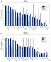
Figure 2. Performance of the algorithms according to Variation of Information (VI), Surprise (S) and Modularity (Q) in LFR and RC benchmarks.
Average performance and standard errors of the mean are shown. Performance values were obtained by the following method: 1) the VI, S or Q values of the partitions provided by the 18 algorithms in each of the networks (i.e. 700 values for LFR benchmarks, 500 values in RC benchmarks) were established; 2) For each network, the algorithms were assigned a rank according to their performance (1 = optimal, 18 = worse); identical ranks were given to tied algorithms (i. e. the ranks that would correspond to each of them were summed up and then divided by the number of tied algorithms); and, 3) Performance was calculated as 18 – average rank, meaning that 17 is the maximum possible value that would obtain an algorithm that outperforms the rest in all networks, and 0 equals to being the worst in all networks.
Figure 3
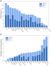
Figure 3. A simple meta-algorithm based on Surprise maximization improves over all known community detection algorithms.
(a) Performances (calculated as in Figure 2) for all the algorithms are compared in both the LFR and the RC benchmarks with the performance of a strategy that consists in picking up the algorithm that provides the highest S value (Smax). (b) For the Smax strategy, the average VI values for the 1200 networks analyzed are very close to zero, i.e. an almost optimal performance.
Figure 4
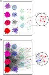
Figure 4. When VI and Surprise maximum values do not coincide, the difference is often due to minimal changes in the community structure of the network.
This is an example from the RC benchmark where Smax > Sorig (see text). a): original structure. b): after R = 10% has been applied. Smax is obtained when a single unit (square) is classified as being isolated from its original 4-nodes community (highlighted). As shown in panel b), the critical unit has become almost fully separated from the rest of the nodes in its original community, only one link remains, while it has been connected to many nodes in other communities.
Figure 5
Figure 5. The performance of the algorithms in the limit cases (μ = 0.7, R = 50%) and beyond those limits (μ = 0.8 – 0.9, R = 60 – 90%) are correlated.
A statistically significant correlation was found, despite the fact that some algorithms, such as Infomap or LPA, totally collapsed. These algorithms established partitions consisting in a single community, which led to VI = 0 when compared with the original distribution.
Figure 6
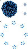
Figure 6. Two extreme networks designed to test the behavior of Surprise when small communities are present.
(a) A network with three communities (sizes 400, 13, 13). The nodes of the largest community have an average degree of 100, while the nodes in the two smallest communities form cliques. The three communities are interconnected by single links, as shown. (b) Cliques, each one with five nodes, which are connected also by single links in a way that can be depicted as a ring. The figure shows an example with eight cliques, but that number was progressively increased to determine whether the partition with highest S still corresponded to the one in which each cliques was an independent community.

Similar articles

Cited by

References

    1. Wasserman S. & Faust K. Social Network Analysis: Methods and Applications. (Cambridge University Press, 1994).
    1. Strogatz S. H. Exploring complex networks. Nature 410, 268–276 (2001). - PubMed
    1. Barabási A.-L. & Oltvai Z. N. Network biology: understanding the cell's functional organization. Nat. Rev. Genet. 5, 101–113 (2004). - PubMed
    1. Costa L. D. F., Rodrigues F. A., Travieso G. & Boas P. R. V. Characterization of complex networks: A survey of measurements. Adv. Phys. 56, 167 (2007).
    1. Newman M. E. J. Networks: An Introduction (Oxford University Press, 2010).

Publication types

LinkOut - more resources